- ...1
- This section was added August 2023 for the next (third) printing of the 2010 edition, since it contains nothing new since 2010, in principle.
.
.
.
.
.
.
.
.
.
.
.
.
.
.
.
.
.
.
.
.
.
.
.
.
.
.
.
.
.
.
- ...2
- This section was added August 2023 for the next (third) printing of the 2010 edition, since it contains nothing new since 2010, in principle.
.
.
.
.
.
.
.
.
.
.
.
.
.
.
.
.
.
.
.
.
.
.
.
.
.
.
.
.
.
.
- ...3
- This section was added August 2023 for the next (third) printing of the 2010 edition, since it contains nothing new since 2010, in principle.
.
.
.
.
.
.
.
.
.
.
.
.
.
.
.
.
.
.
.
.
.
.
.
.
.
.
.
.
.
.
- ...4
- This section was added August 2023 for the next (third) printing of the 2010 edition, since it contains nothing new since 2010, in principle.
.
.
.
.
.
.
.
.
.
.
.
.
.
.
.
.
.
.
.
.
.
.
.
.
.
.
.
.
.
.
- ...
email1.1
- jos at ccrma
.
.
.
.
.
.
.
.
.
.
.
.
.
.
.
.
.
.
.
.
.
.
.
.
.
.
.
.
.
.
- ... performance.2.1
- This distinction
is also important when evaluating real-world musical instruments.
It is better to ask a skilled performer to comment on the quality of
an instrument than a listener. A good musician can make almost any
instrument sound good, while appreciating its defects and working
around them in performance.
.
.
.
.
.
.
.
.
.
.
.
.
.
.
.
.
.
.
.
.
.
.
.
.
.
.
.
.
.
.
- ...
pianos''.2.2
- For example, the Synthogy Ivory (a $349
software product in 2006), ships as 40 Gigabytes on ten DVDs (three
sampled pianos). Every key is sampled, with 4-10 ``velocity
layers'', separate recordings with the soft pedal down, and separate
``release'' recordings, for multiple striking velocities. (Source:
Electronic Musician magazine, October 2006)
.
.
.
.
.
.
.
.
.
.
.
.
.
.
.
.
.
.
.
.
.
.
.
.
.
.
.
.
.
.
- ... acoustic2.3
- In the case of audio effects,
``acoustic'' recordings are normally replaced by ``electronic''
recordings. The same applies to the sampling of vintage electronic
instruments, such as the Fender Rhodes electric piano, etc.
.
.
.
.
.
.
.
.
.
.
.
.
.
.
.
.
.
.
.
.
.
.
.
.
.
.
.
.
.
.
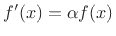
- ... equation2.4
- See
Appendix B for further discussion of Newton's laws of motion.
.
.
.
.
.
.
.
.
.
.
.
.
.
.
.
.
.
.
.
.
.
.
.
.
.
.
.
.
.
.
- ...2.5
- Digitizing a system generally means
converting it from continuous-time to discrete-time form. For an
ODE, for example, this typically involves algebraically replacing
the time differential
 in the ODE by a practical sampling
interval
in the ODE by a practical sampling
interval  , as will be discussed below and in §7.3.1.
.
.
.
.
.
.
.
.
.
.
.
.
.
.
.
.
.
.
.
.
.
.
.
.
.
.
.
.
.
.
- ... dashpot2.6
- A
dashpot is the idealized mechanical equivalent of a
resistor in electrical circuit theory. Its compression-velocity
is proportional to applied force, i.e.,
 .
Dashpots are often used to model forces due to friction and
are typically valid over a restricted frequency range. Masses and
springs are mechanical equivalents of electrical inductors and
capacitors, respectively. More about these elements will be
discussed below in this chapter and later in this book.
.
.
.
.
.
.
.
.
.
.
.
.
.
.
.
.
.
.
.
.
.
.
.
.
.
.
.
.
.
.
- ....2.7
- Transverse displacement
is displacement in a plane orthogonal to the string axis
 .
.
.
.
.
.
.
.
.
.
.
.
.
.
.
.
.
.
.
.
.
.
.
.
.
.
.
.
.
.
.
.
- ... beyond.2.8
- It is interesting to note that in the
development of quantum mechanics in the early 1900s, it was
necessary to replace deterministic Newtonian dynamics with a
probabilistic model. In quantum mechanics, probability
distributions may follow deterministic trajectories as in Newtonian
mechanics (see, for example, Schrödinger's equation), but they are
only probability distributions, so there is no deterministic ``clock
works'' at the smallest physical scales. We are fortunate to be able
to use Newtonian dynamics with such great accuracy. Our difficulty will
be complexity, not randomness. Paradoxically, the typical way to
deal with overwhelming complexity is to model it as random (e.g.,
filtered white noise).
.
.
.
.
.
.
.
.
.
.
.
.
.
.
.
.
.
.
.
.
.
.
.
.
.
.
.
.
.
.
- ....2.9
- As discussed in §1.3.6, only velocity
 is
needed for the state variable of a mass, since a mass moving in one
dimension has only one degree of freedom (with energy
is
needed for the state variable of a mass, since a mass moving in one
dimension has only one degree of freedom (with energy  ).
However, since it is physically reasonable to expect both velocity
and position to be needed for the state of a point mass, let's
``play that out'' and see how it goes. This also gives us a simple
vector example to study.
).
However, since it is physically reasonable to expect both velocity
and position to be needed for the state of a point mass, let's
``play that out'' and see how it goes. This also gives us a simple
vector example to study.
.
.
.
.
.
.
.
.
.
.
.
.
.
.
.
.
.
.
.
.
.
.
.
.
.
.
.
.
.
.
- ... proper2.10
- See
[452, p. 133] regarding the cases
 for which a
``long division'' is first performed to obtain an FIR part in
parallel with a strictly proper part.
for which a
``long division'' is first performed to obtain an FIR part in
parallel with a strictly proper part.
.
.
.
.
.
.
.
.
.
.
.
.
.
.
.
.
.
.
.
.
.
.
.
.
.
.
.
.
.
.
- ... diagonal.2.11
- More precisely,
 is diagonal when the
poles are distinct. A repeated pole can result in a block of
having 1s along its superdiagonal.
is diagonal when the
poles are distinct. A repeated pole can result in a block of
having 1s along its superdiagonal.
.
.
.
.
.
.
.
.
.
.
.
.
.
.
.
.
.
.
.
.
.
.
.
.
.
.
.
.
.
.
- ... eigenvectors.2.12
- A
generalized eigenvector
 of matrix
corresponding to
eigenvalue
of matrix
corresponding to
eigenvalue  having multiplicity
  is a nonzero solution
of
is a nonzero solution
of
 .
.
.
.
.
.
.
.
.
.
.
.
.
.
.
.
.
.
.
.
.
.
.
.
.
.
.
.
.
.
.
.
- ... zero.2.13
- The other law routinely used in
circuit analysis is that the sum of all currents entering a
circuit node (connection of wires) is zero. This kind of
analysis will be revisited in §9.3.1.
.
.
.
.
.
.
.
.
.
.
.
.
.
.
.
.
.
.
.
.
.
.
.
.
.
.
.
.
.
.
- ... resistance.2.14
- Note that models of damping in
practical physical systems are rarely completely independent of
frequency, as is the ideal dashpot.
.
.
.
.
.
.
.
.
.
.
.
.
.
.
.
.
.
.
.
.
.
.
.
.
.
.
.
.
.
.
- ...JOSFP2.15
- For a short online introduction to Laplace transforms, see, e.g.,
http://ccrma.stanford.edu/~jos/filters/Laplace_Transform_Analysis.html.
.
.
.
.
.
.
.
.
.
.
.
.
.
.
.
.
.
.
.
.
.
.
.
.
.
.
.
.
.
.
- ... direction.3.1
- To determine whether a surface is
effectively flat, it may first be smoothed so that variations less
than a wavelength in size are ignored. That is, waves do not ``see''
variations on a scale much less than a wavelength.
.
.
.
.
.
.
.
.
.
.
.
.
.
.
.
.
.
.
.
.
.
.
.
.
.
.
.
.
.
.
- ...STK4.3.2
- In the code of Fig.2.10, the first executable line
changes the global STK sampling-rate from 44100 Hz (the default) to
that of the input soundfile. If this is not done, there is a hidden
sampling-rate conversion using linear interpolation when the input
file is read, if its sampling rate is different from the global STK
sampling-rate. This default rate conversion could alternatively be
canceled by saying input.setRate(1.0); after the input file
is opened.
.
.
.
.
.
.
.
.
.
.
.
.
.
.
.
.
.
.
.
.
.
.
.
.
.
.
.
.
.
.
- ....3.3
- It is easy to see that the exponential function
 has the property
 . To show that all
differentiable functions with this property are exponentials, one can
look at the definition of the derivative of
. To show that all
differentiable functions with this property are exponentials, one can
look at the definition of the derivative of  with respect to
:
with respect to
:
Since
 , we must have
  . Therefore, the last
limit above converges to some constant
. Therefore, the last
limit above converges to some constant
 , and
, and
 . In this way, it is shown that
  satisfies a differential equation whose solution space consists of
exponential functions of the form
satisfies a differential equation whose solution space consists of
exponential functions of the form
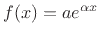 , and to obtain
, we must have
, and to obtain
, we must have  .
.
.
.
.
.
.
.
.
.
.
.
.
.
.
.
.
.
.
.
.
.
.
.
.
.
.
.
.
.
.
.
- ...
dispersion3.4
- Dispersion occurs in a
traveling wave whenever the propagation speed is different at two or
more frequencies.
.
.
.
.
.
.
.
.
.
.
.
.
.
.
.
.
.
.
.
.
.
.
.
.
.
.
.
.
.
.
- ... equal.3.5
- The signs may differ, however. For
example, imagine twisting a stretched string about a point
along its length in the plane of transverse vibration. In that
case, the transverse-displacement pulses propagating away from the
twist have opposite sign. This opposite-sign effect happens also
for slope waves emanating from a pluck disturbance, as we'll
see in Chapter 6. (A positive pluck corresponds to a
positive slope on its left and a negative slope on its right.)
.
.
.
.
.
.
.
.
.
.
.
.
.
.
.
.
.
.
.
.
.
.
.
.
.
.
.
.
.
.
- ... law3.6
- Newton's third law states that ``every
action produces an equal and opposite reaction.'' Therefore, every
``physical'' signal connection must be bidirectional, in
order to model both the applied force and the equal reaction force,
or ``loading effect''. Bidirectional signal connections are
typically called ports. A ``port'' (one physical
connection point) in electrical circuit theory consists of two
variables, typically voltage and current. In acoustics,
corresponding port variables would be pressure and velocity. As
discussed later (e.g., for Wave Digital Filters in Appendix F), a
simple 2x2 matrix linear transformation converts ``force and flow''
port variables, such as these, to ``traveling-wave component'' port
variables.
.
.
.
.
.
.
.
.
.
.
.
.
.
.
.
.
.
.
.
.
.
.
.
.
.
.
.
.
.
.
- ...
waves3.7
- Loading effects can be viewed as the result of
instantaneous return waves. This equivalence is seen clearly, for
example, in Wave Digital Filters (Appendix F).
.
.
.
.
.
.
.
.
.
.
.
.
.
.
.
.
.
.
.
.
.
.
.
.
.
.
.
.
.
.
- ...
neglected.3.8
- This follows years of standard practice in analog
electric circuit design using voltage transfer
interconnections. For ``voltage transfer'' from one circuit-stage
to another with minimized loading effects, output impedances are
made as low as practical, while input impedances are set very high.
For example, in analog synthesizers built during the 1970s, input
impedances were typically around 100 times output impedances (e.g.,
100K and 1K Ohms, respectively in a typical op-amp circuit)
[205].
.
.
.
.
.
.
.
.
.
.
.
.
.
.
.
.
.
.
.
.
.
.
.
.
.
.
.
.
.
.
- ... as3.9
- Note that
Fig.2.24 is given in direct form 2, so its describing equations are
 . To make the figure
correspond exactly to the direct-form-1 difference equation, simply
move
. To make the figure
correspond exactly to the direct-form-1 difference equation, simply
move  from the output arrow to the input arrow. That is, commute
the scaling by
and the feedback loop so that
is first.
from the output arrow to the input arrow. That is, commute
the scaling by
and the feedback loop so that
is first.
.
.
.
.
.
.
.
.
.
.
.
.
.
.
.
.
.
.
.
.
.
.
.
.
.
.
.
.
.
.
- ... filter|textbf,3.10
- Readers of the main chapters of this book are not
required to know linear algebra, but one does not have to learn much
to follow the discussion in this section. See, for example,
[454, available online] for the basic matrix operations. An
excellent linear algebra text is [332]. See also the lecture
videos by Strang by searching for ``linear algebra'' at
http://ocw.mit.edu/.
.
.
.
.
.
.
.
.
.
.
.
.
.
.
.
.
.
.
.
.
.
.
.
.
.
.
.
.
.
.
- ....3.11
- If
 is complex, transposition must include
complex conjugation, i.e.,
is complex, transposition must include
complex conjugation, i.e.,
 . The
conjugate-transpose
. The
conjugate-transpose
 is called the Hermitian
transpose of
.
is called the Hermitian
transpose of
.
.
.
.
.
.
.
.
.
.
.
.
.
.
.
.
.
.
.
.
.
.
.
.
.
.
.
.
.
.
.
- ...
1,3.12
- By definition,
 , so that all singular values
of an orthogonal matrix are equal to 1.
, so that all singular values
of an orthogonal matrix are equal to 1.
.
.
.
.
.
.
.
.
.
.
.
.
.
.
.
.
.
.
.
.
.
.
.
.
.
.
.
.
.
.
- ... line.3.13
- This
structure may be quickly derived by forming a series combination of a
feedback comb filter followed by a feedforward comb filter, and
noticing that the two delay lines contain the same numbers at all
times. Therefore, the two delay lines can be replaced by a single
shared delay line.
.
.
.
.
.
.
.
.
.
.
.
.
.
.
.
.
.
.
.
.
.
.
.
.
.
.
.
.
.
.
- ...causal|textbf3.14
- A filter is said
to be causal if its impulse response
 is zero for
  .
.
.
.
.
.
.
.
.
.
.
.
.
.
.
.
.
.
.
.
.
.
.
.
.
.
.
.
.
.
.
.
- ...fbffcf.3.15
- Gerzon's starting point was Schroeder's
allpass which differs slightly from Eq.(2.15), having difference
equation [415]
with  required for stability. This structure can be derived
from Eq.(2.15) on page
required for stability. This structure can be derived
from Eq.(2.15) on page ![[*]](../icons/crossref.png) by moving the feedforward path to
the other side of the input summer and deriving the new gain for
by moving the feedforward path to
the other side of the input summer and deriving the new gain for
 . Gerzon's idea was to replace the
  -sample delay by a
multi-input, multi-output (MIMO) allpass-filter matrix;
Gerzon's ``unitary frequency-response matrices'' correspond to
paraunitary matrix transfer functions
[452, Appendix D].
-sample delay by a
multi-input, multi-output (MIMO) allpass-filter matrix;
Gerzon's ``unitary frequency-response matrices'' correspond to
paraunitary matrix transfer functions
[452, Appendix D].
.
.
.
.
.
.
.
.
.
.
.
.
.
.
.
.
.
.
.
.
.
.
.
.
.
.
.
.
.
.
- ... matrix|textbf3.16
- A (possibly complex) matrix
 is said to be
unitary if
is said to be
unitary if
 , where
 is the Hermitian transpose of
  . A real
unitary matrix is said to be orthogonal, which is the case
most commonly used in practice.
. A real
unitary matrix is said to be orthogonal, which is the case
most commonly used in practice.
.
.
.
.
.
.
.
.
.
.
.
.
.
.
.
.
.
.
.
.
.
.
.
.
.
.
.
.
.
.
- ... impedance3.17
-
See §7.1 for definitions and discussion regarding
impedance.
.
.
.
.
.
.
.
.
.
.
.
.
.
.
.
.
.
.
.
.
.
.
.
.
.
.
.
.
.
.
- ... ear,4.1
- One tapped
delay line can also model one source to multiple ears, or vice versa
(Fig.5.6).
.
.
.
.
.
.
.
.
.
.
.
.
.
.
.
.
.
.
.
.
.
.
.
.
.
.
.
.
.
.
- ... time4.2
- Reverberation time is
typically defined as
 ,
the time, in seconds, to decay by 60 dB.
,
the time, in seconds, to decay by 60 dB.
.
.
.
.
.
.
.
.
.
.
.
.
.
.
.
.
.
.
.
.
.
.
.
.
.
.
.
.
.
.
- ... shown4.3
- A simple proof for rectangular rooms can be based on
considering a single spherical wave produced from a point source in
the room. Imagine tesselating all of 3D space with copies of the
original room (minus the source), all in the same orientation. As
the spherical wave expands, it intersects a number of rooms that is
roughly proportional to its radius squared. Since the radius is
proportional to time for an expanding spherical wavefront (
 ),
the number of rooms containing a wave section grows as
),
the number of rooms containing a wave section grows as  . By
adding all the rooms together (flipping every other one along
and
. By
adding all the rooms together (flipping every other one along
and  ), we obtain the acoustic field in the original reverberant
room at time
), we obtain the acoustic field in the original reverberant
room at time  , for the case of lossless wall reflections of
pressure waves. (This is the dual of the usual image method
for computing the impulse response of a room
[11].) Since each wave-section traverses each
point exactly once in each room image (disregarding reflections,
which are accounted for by different room images), the number of
echoes at any point in the room during the time it takes a plane
wave to traverse the room is very close to the number of wave
sections in the room at the beginning of that time interval.
Incidentally, this construction gives, in the limit as
, for the case of lossless wall reflections of
pressure waves. (This is the dual of the usual image method
for computing the impulse response of a room
[11].) Since each wave-section traverses each
point exactly once in each room image (disregarding reflections,
which are accounted for by different room images), the number of
echoes at any point in the room during the time it takes a plane
wave to traverse the room is very close to the number of wave
sections in the room at the beginning of that time interval.
Incidentally, this construction gives, in the limit as
 ,
a derivation and vivid visualization of the diffuse
field--the superposition of equal-amplitude traveling
plane-waves arriving from all directions and having uniformally
distributed random arrival phase [352,47].
,
a derivation and vivid visualization of the diffuse
field--the superposition of equal-amplitude traveling
plane-waves arriving from all directions and having uniformally
distributed random arrival phase [352,47].
.
.
.
.
.
.
.
.
.
.
.
.
.
.
.
.
.
.
.
.
.
.
.
.
.
.
.
.
.
.
- ... shown4.4
- As described in virtually any acoustics textbook, the resonant modes of a
rectangular room are given by (see, e.g., [352, pp. 284-286])
 |
(4.1) |
where
 denotes the
  th harmonic frequency (radian/meter)
of the fundamental standing wave in the
direction (
th harmonic frequency (radian/meter)
of the fundamental standing wave in the
direction ( being the
length of the room along
), and similarly for the
and
being the
length of the room along
), and similarly for the
and  directions. Thus, the mode frequencies of a room can be enumerated on
a uniform 3D Cartesian grid indexed by
directions. Thus, the mode frequencies of a room can be enumerated on
a uniform 3D Cartesian grid indexed by  . The grid spacings
along
,
, and
are taken to be
. The grid spacings
along
,
, and
are taken to be  ,
,  , and
, and
 , respectively. From Eq.(3.1), the spatial frequency
of mode
is given by the distance from the origin
of the grid to the point indexed by
. Therefore, the number of room
modes having spatial frequency between
and
, respectively. From Eq.(3.1), the spatial frequency
of mode
is given by the distance from the origin
of the grid to the point indexed by
. Therefore, the number of room
modes having spatial frequency between
and  is equal to
the number of grid points lying in the spherical annulus between
radius
and
. Since the grid is uniform, this number
grows as
is equal to
the number of grid points lying in the spherical annulus between
radius
and
. Since the grid is uniform, this number
grows as  .
.
.
.
.
.
.
.
.
.
.
.
.
.
.
.
.
.
.
.
.
.
.
.
.
.
.
.
.
.
.
.
- ...4.5
- One definition of when late
reverberation begins is when it begins to look Gaussian, since
a random sum of plane waves uniformly distributed over all angles of
arrival yields a Gaussian distributed pressure field. (The fact that
late reverberation in a rectangular room always approaches the diffuse field--a
superposition of plane waves traveling in all directions can be seen
from the ``image-method dual'' argument in §3.2.1.) One way to
test for Gaussianness is to form a histogram of impulse
response sample values over a finite window (say 10ms, or roughly 500
samples), and compare the normalized histogram
 to a standard
Gaussian bell curve
to a standard
Gaussian bell curve  computed using the measured sample
variance. A threshold can be placed on
computed using the measured sample
variance. A threshold can be placed on
 , or some
number of higher order sample moments can be compared. A simpler test
is to determine when roughly 30% of the samples in a frame have
magnitude larger than one standard deviation (
, or some
number of higher order sample moments can be compared. A simpler test
is to determine when roughly 30% of the samples in a frame have
magnitude larger than one standard deviation (
 )
[3],
since the probability of this occurring in truly Gaussian sequences is
)
[3],
since the probability of this occurring in truly Gaussian sequences is
 erf
erf , where
erf
, where
erf denotes the ``error function'' (integral from
  to
of the
Gaussian probability density function with normalized variance
to
of the
Gaussian probability density function with normalized variance
 ). For a zero-mean signal
  , the sample standard
deviation
, the sample standard
deviation  is given by the root-mean-square (RMS level).
Another
desired property of ``late reverb'' is that the remaining energy in
the impulse response (Schroeder's Energy Decay Curve (EDC)
[416]), has begun what appears to be an
exponential decay. This can be ascertained by fitting an exponential
to the EDC using, e.g., Prony's method.
is given by the root-mean-square (RMS level).
Another
desired property of ``late reverb'' is that the remaining energy in
the impulse response (Schroeder's Energy Decay Curve (EDC)
[416]), has begun what appears to be an
exponential decay. This can be ascertained by fitting an exponential
to the EDC using, e.g., Prony's method.
.
.
.
.
.
.
.
.
.
.
.
.
.
.
.
.
.
.
.
.
.
.
.
.
.
.
.
.
.
.
- ... (TDL).4.6
- This idea was apparently first suggested by
Schroeder in 1970 [418] and evidently first implemented
by Moorer [317].
.
.
.
.
.
.
.
.
.
.
.
.
.
.
.
.
.
.
.
.
.
.
.
.
.
.
.
.
.
.
- ...MoorerReverb79.4.7
- In computer music, an old trick
for making a synthesized tone sound reverberated is to randomly modulate
its amplitude envelope, and to append a low-level exponentially decaying
tail to the amplitude envelope (also modulated). This can produce a very
convincing illusion.
.
.
.
.
.
.
.
.
.
.
.
.
.
.
.
.
.
.
.
.
.
.
.
.
.
.
.
.
.
.
- ...
examples.4.8
- https://ccrma.stanford.edu/~jos/wav/FM-BrassCanon2.wav
.
.
.
.
.
.
.
.
.
.
.
.
.
.
.
.
.
.
.
.
.
.
.
.
.
.
.
.
.
.
- ....4.9
- As
an alternative to the output delay values shown in Fig.3.7,
the values
![$ [0.013, 0.011, 0.019, 0.017]f_s$](img722.png) have been used.
have been used.
.
.
.
.
.
.
.
.
.
.
.
.
.
.
.
.
.
.
.
.
.
.
.
.
.
.
.
.
.
.
- ... alone.4.10
- There is a Freeverb
pd ``external'' in both the pd-extended and
faust-pd packages, and it appears in the muse
sequencer, kdemultimedia, clm, and faust
language packages, all included with Planet CCRMA. Other versions may
be found by a Web search for ``Freeverb source'', but I have not found
any version that isn't essentially the same June 2000 version by Jezar
at Dreampoint.
.
.
.
.
.
.
.
.
.
.
.
.
.
.
.
.
.
.
.
.
.
.
.
.
.
.
.
.
.
.
- ...
(LBCF4.11
- ``Lowpass-Back-Comb-Filter''--to keep all the
comb-filter acronyms down to four characters: FFCF, FBCF, LBCF.
Author's prerogative!
.
.
.
.
.
.
.
.
.
.
.
.
.
.
.
.
.
.
.
.
.
.
.
.
.
.
.
.
.
.
- ...math.lib4.12
- Details about
Faust may be found at
http://faust.grame.fr/.
.
.
.
.
.
.
.
.
.
.
.
.
.
.
.
.
.
.
.
.
.
.
.
.
.
.
.
.
.
.
- ... diagonal.4.13
- This is easy to
show by performing an expansion by minors to calculate
 , always choosing to expand along the top row (for lower
triangular) or first column (for upper triangular).
, always choosing to expand along the top row (for lower
triangular) or first column (for upper triangular).
.
.
.
.
.
.
.
.
.
.
.
.
.
.
.
.
.
.
.
.
.
.
.
.
.
.
.
.
.
.
- ...
repeats.4.14
- Fritz Menzer, in ``Choosing Optimal Delays for Feedback Delay Networks'',
http://pub.dega-akustik.de/DAGA_2014/data/articles/000025.pdf, found
that ``using mutually prime delays [in FDNs] avoids only a negligible
subset of echo superpositions'', and proposed free optimization of the
delay lengths to achieve desired qualities.
.
.
.
.
.
.
.
.
.
.
.
.
.
.
.
.
.
.
.
.
.
.
.
.
.
.
.
.
.
.
- ...4.15
- This substitution was first applied
to complete reverberators by Jot [217,218]. The
idea is closely related to the approximate pole analysis in
[317, p. 17], [432, pp. 170-172],
and [208], and somewhat also to the allpass conformal
maps used in [318,461].
.
.
.
.
.
.
.
.
.
.
.
.
.
.
.
.
.
.
.
.
.
.
.
.
.
.
.
.
.
.
- ...FDNJot).4.16
- Note that, as
developed here, the delay-line filters
 should be located
either before or after its associated delay line, while
Fig.3.10 associates it with the feedback matrix. The
difference is typically not audible.
should be located
either before or after its associated delay line, while
Fig.3.10 associates it with the feedback matrix. The
difference is typically not audible.
.
.
.
.
.
.
.
.
.
.
.
.
.
.
.
.
.
.
.
.
.
.
.
.
.
.
.
.
.
.
- ... dc.4.17
- In a Faust
implementation, this form was found to be more numerically sensitive
than that of the previous section when changing the
s in
real time (see §3.7.9).
.
.
.
.
.
.
.
.
.
.
.
.
.
.
.
.
.
.
.
.
.
.
.
.
.
.
.
.
.
.
- ... FOSS4.18
- FOSS
 Free Open Source Software
.
.
.
.
.
.
.
.
.
.
.
.
.
.
.
.
.
.
.
.
.
.
.
.
.
.
.
.
.
.
- ...zita-rev1,4.19
- http://kokkinizita.linuxaudio.org/linuxaudio/zita-rev1-doc/quickguide.html
.
.
.
.
.
.
.
.
.
.
.
.
.
.
.
.
.
.
.
.
.
.
.
.
.
.
.
.
.
.
- ...JOSFP,4.20
- https://ccrma.stanford.edu/~jos/filters/Low_High_Shelving_Filters.html
.
.
.
.
.
.
.
.
.
.
.
.
.
.
.
.
.
.
.
.
.
.
.
.
.
.
.
.
.
.
- ...
respectively.4.21
- This section describes the Faust version
zita_rev1, which may not be exactly the same as the
C++ version zita-rev1, although each control parameter
range is the same, and the filter-orders are the same, so at least
near-equivalance is expected.
.
.
.
.
.
.
.
.
.
.
.
.
.
.
.
.
.
.
.
.
.
.
.
.
.
.
.
.
.
.
- ...Kendall84.4.22
- Of course, correct angles-of-arrival
for early reflections are more straightforward to implement using an
array of loudspeakers enclosing the listener.
.
.
.
.
.
.
.
.
.
.
.
.
.
.
.
.
.
.
.
.
.
.
.
.
.
.
.
.
.
.
- ...5.1
- A causal IIR filter can be used for random-access table
lookup by simply starting the filter at a point sufficiently far
away in the table and ``running it'' until it reaches steady-state
at the desired interpolation point. While this requires at least as
many multiply-adds as an FIR filter spanning the same duration, the
number of IIR filter coefficients can be much less than the number
of FIR filter coefficients required. IIR interpolators are therefore
possibly interesting for certain memory-starved VLSI applications.
.
.
.
.
.
.
.
.
.
.
.
.
.
.
.
.
.
.
.
.
.
.
.
.
.
.
.
.
.
.
- ... samples.5.2
- Classically, an interpolation
 of discrete data points
  always required
 ;
that is, the interpolating function must always pass through the given
data points. More recently, however, particularly in the field of
computer graphics, interpolation schemes such as Bezier splines
have been defined which do not always pass through the known points.
;
that is, the interpolating function must always pass through the given
data points. More recently, however, particularly in the field of
computer graphics, interpolation schemes such as Bezier splines
have been defined which do not always pass through the known points.
.
.
.
.
.
.
.
.
.
.
.
.
.
.
.
.
.
.
.
.
.
.
.
.
.
.
.
.
.
.
- ... matlab:5.3
- Say ``help;'' within maxima
and/or ``man maxima'' in a shell to get started. Emacs users
should say ``M-x maxima''.
.
.
.
.
.
.
.
.
.
.
.
.
.
.
.
.
.
.
.
.
.
.
.
.
.
.
.
.
.
.
- ...5.4
- To see this, consider that a unit-amplitude sinusoid at half
the sampling rate
 is either
  or
or  . Therefore,
the frequency response
. Therefore,
the frequency response  of every real filter at
is
a real number
of every real filter at
is
a real number
 that is either positive or negative (or
zero). When
that is either positive or negative (or
zero). When  , the filter's phase delay must be an even integer
number of samples. When
, the filter's phase delay must be an even integer
number of samples. When  , the filter delay is constrained to be
some odd number of samples. Taken together, the possible delays at
for real filters are the integers. The particular integer is
obtained by finding the limit as
, the filter delay is constrained to be
some odd number of samples. Taken together, the possible delays at
for real filters are the integers. The particular integer is
obtained by finding the limit as
 . The case
  can be
associated with a non-integer limit, as suggested by the line for
can be
associated with a non-integer limit, as suggested by the line for
 samples delay in Fig.4.18 above, and as easily
shown analytically for order 1 (simple linear interpolation with
coefficients
samples delay in Fig.4.18 above, and as easily
shown analytically for order 1 (simple linear interpolation with
coefficients  , corresponding to a desired delay of
  samples) [452].
.
.
.
.
.
.
.
.
.
.
.
.
.
.
.
.
.
.
.
.
.
.
.
.
.
.
.
.
.
.
- ...VesaT.5.5
- http://www.acoustics.hut.fi/~vpv/publications/vesan_vaitos/ch3_pt2_lagrange.pdf
.
.
.
.
.
.
.
.
.
.
.
.
.
.
.
.
.
.
.
.
.
.
.
.
.
.
.
.
.
.
- ... rule,5.6
- Evaluation of a polynomial
 by Horner's rule can be expressed as
 .
.
.
.
.
.
.
.
.
.
.
.
.
.
.
.
.
.
.
.
.
.
.
.
.
.
.
.
.
.
.
.
- ....5.7
- Of course, all derivatives of
must
be calculated from the underlying continuous signal
 represented by the samples
and then evaluated at
represented by the samples
and then evaluated at  .
.
.
.
.
.
.
.
.
.
.
.
.
.
.
.
.
.
.
.
.
.
.
.
.
.
.
.
.
.
.
.
- ...JOSFP.5.8
- To see this, note that the integral of the
group delay around the unit circle is simply minus the winding
number of the phase response (the number of zeros minus the number of
poles inside the unit circle):
By the graphical method for phase response calculation [452, Chapter
8], each zero contributes  radians to
 , and each pole contributes
  radians. Thus,
the average group delay around the unit circle is
radians. Thus,
the average group delay around the unit circle is
.
.
.
.
.
.
.
.
.
.
.
.
.
.
.
.
.
.
.
.
.
.
.
.
.
.
.
.
.
.
- ...
processing.5.9
- The material in this section was adapted from
https://ccrma.stanford.edu/~jos/resample/,
which is an updated online version of [464].
.
.
.
.
.
.
.
.
.
.
.
.
.
.
.
.
.
.
.
.
.
.
.
.
.
.
.
.
.
.
- ... kHz.5.10
- We arbitrarily define the
 % guard band as a
percentage of half the sampling rate actually used, not as
% of the
desired
kHz bandwidth which would call for a
% guard band as a
percentage of half the sampling rate actually used, not as
% of the
desired
kHz bandwidth which would call for a  kHz sampling rate.
.
.
.
.
.
.
.
.
.
.
.
.
.
.
.
.
.
.
.
.
.
.
.
.
.
.
.
.
.
.
- ...Bartlett70,SmithAllpassFlanger,Bode84,Anderton85,Dattorro97,Keen99.6.1
- Flanging was apparently invented independently several
times. According to http://www.geofex.com/Article_Folders/phasers/phase.html, the
flanging technique was discovered by Phil Spectre in the 1950s in the
context of trying to ``thicken'' a vocal track by summing two copies
of a track variably delayed in this way. His first use of flanging as
an effect is said to be in his song ``The Big Hurt''.
According to historian Mark Lewisohn [288], as summarized
at http://en.wikipedia.org/wiki/Flanging
(accessed March 28, 2010), the
term ``flanging'' was coined by John Lennon of the Beatles to describe
what EMI engineer Ken Townsend called ``Artificial Double Tracking''
(ADT). ADT was said to be developed by Townsend in response to John
Lennon's request to try to eliminate the work of recording vocal
tracks twice in order to ``double'' them. George Martin has said to
have explained the effect as follows: ``Now listen, it's very
simple. We take the original image and we split it through a
double-bifurcated sploshing flange with double negative feedback.''
[288]. This suggests that negative regenerative feedback
was used in the original stereo flanging technique
(§2.6.2). The first Beatles track using flanging is
said to have been ``Tomorrow Never Knows'' on the Revolver album
(recorded April 6, 1966). Perhaps the most obvious early example of
flanging was in the popular song ``Itchykoo Park'' by The Small Faces
(1967); this instance is said to have originated with engineer George
Chkiantz at Olympic Studios in London. The song featured a foreground
drum-roll on a snare with strong flanging throughout, and the vocals
were flanged as well.
.
.
.
.
.
.
.
.
.
.
.
.
.
.
.
.
.
.
.
.
.
.
.
.
.
.
.
.
.
.
- ... sound.6.2
- For sound
examples, see
http://www.harmony-central.com/Effects/Articles/Flanging/.
.
.
.
.
.
.
.
.
.
.
.
.
.
.
.
.
.
.
.
.
.
.
.
.
.
.
.
.
.
.
- ...notches6.3
- The term notch here refers to the
elimination of sound energy at a single frequency or over a narrow
frequency interval. Another term for this is ``null''.
.
.
.
.
.
.
.
.
.
.
.
.
.
.
.
.
.
.
.
.
.
.
.
.
.
.
.
.
.
.
- ...Bartlett70,6.4
- According to
http://www.eventide.com/About/History.aspx,
a dual 200 ms delay-line for simulating flanging was called the
Instant Phaser. This was the first commercial product circa
1970 made by Eventide Corp. (better known as makers of the
Harmonizer).
.
.
.
.
.
.
.
.
.
.
.
.
.
.
.
.
.
.
.
.
.
.
.
.
.
.
.
.
.
.
- ... notches.6.5
- The
author discovered this first-hand by looking at the circuit for the
MXR phase shifter in 1975.
.
.
.
.
.
.
.
.
.
.
.
.
.
.
.
.
.
.
.
.
.
.
.
.
.
.
.
.
.
.
- ...SmithEtAlDAFx02.6.6
- https://ccrma.stanford.edu/~jos/doppler/
.
.
.
.
.
.
.
.
.
.
.
.
.
.
.
.
.
.
.
.
.
.
.
.
.
.
.
.
.
.
- ...eq:dopplershift).6.7
- If the tape travels in a loop,
then Fig.5.4 provides a model for the Echoplex (Maestro,
1960), which consists of a tape loop with a fixed write-head and
movable read-head.
.
.
.
.
.
.
.
.
.
.
.
.
.
.
.
.
.
.
.
.
.
.
.
.
.
.
.
.
.
.
- ... first6.8
- The ``first'' write-pointer is defined as the
one writing farthest ahead in time; it must overwrite memory, instead
of summing into it, when a circular buffer is being used, as is
typical.
.
.
.
.
.
.
.
.
.
.
.
.
.
.
.
.
.
.
.
.
.
.
.
.
.
.
.
.
.
.
- ... Leslie,6.9
- http://en.wikipedia.org/wiki/Leslie_speaker
.
.
.
.
.
.
.
.
.
.
.
.
.
.
.
.
.
.
.
.
.
.
.
.
.
.
.
.
.
.
- ... accurate.6.10
- See also
the Hammond Leslie FAQ at
http://www.theatreorgans.com/hammond/faq/files/hammond-faq.pdf
.
.
.
.
.
.
.
.
.
.
.
.
.
.
.
.
.
.
.
.
.
.
.
.
.
.
.
.
.
.
- ...SmithEtAlDAFx02.6.11
- https://ccrma.stanford.edu/~jos/doppler/
.
.
.
.
.
.
.
.
.
.
.
.
.
.
.
.
.
.
.
.
.
.
.
.
.
.
.
.
.
.
- ...dAlembert7.1
- See §A.1 for more about the
history of the wave equation and its traveling-wave solution.
.
.
.
.
.
.
.
.
.
.
.
.
.
.
.
.
.
.
.
.
.
.
.
.
.
.
.
.
.
.
- ... derivation)7.2
- Note that
 and
and  , as
defined, are traveling-wave components of the force acting to
the right on the string. That is, their sum
, as
defined, are traveling-wave components of the force acting to
the right on the string. That is, their sum
 is
physically the force that the string-segment to the left of
position
applies (in the upward direction) to the string-segment
to the right of point
. In other words,
is
physically the force that the string-segment to the left of
position
applies (in the upward direction) to the string-segment
to the right of point
. In other words,  denotes
the vertical force applied by the left segment to the right segment at
time
and position
; thus, it ``acts to the right'', even though
its traveling-wave components,
and
, travel to the left and
right, respectively, at speed
denotes
the vertical force applied by the left segment to the right segment at
time
and position
; thus, it ``acts to the right'', even though
its traveling-wave components,
and
, travel to the left and
right, respectively, at speed  . The net physical force acting to
the right at each point is exactly canceled by an equal and opposite
force acting to the left at each point
. See §C.7.2
for a detailed derivation.
. The net physical force acting to
the right at each point is exactly canceled by an equal and opposite
force acting to the left at each point
. See §C.7.2
for a detailed derivation.
.
.
.
.
.
.
.
.
.
.
.
.
.
.
.
.
.
.
.
.
.
.
.
.
.
.
.
.
.
.
- ... inversion:7.3
- All wave phenomena involve two physical state
variables--one force-like and the other velocity-like. When one of
these variables reflects from a termination with a sign inversion, the
other reflects with no sign inversion, and vice versa. In acoustic
systems, the force-like variable is pressure, and the velocity-like
variable is either particle velocity (in open air) or volume velocity
(in acoustic tubes), as described in §6.2 above. In
electromagnetic systems, the state variables are electric and magnetic
field strengths or voltage and current. In a mass-spring oscillator,
we may choose the velocity and acceleration of the mass as the
coordinates of our state space, or position and velocity. For
transverse waves on vibrating strings, it is usually preferable to use
force and velocity waves as described above.
.
.
.
.
.
.
.
.
.
.
.
.
.
.
.
.
.
.
.
.
.
.
.
.
.
.
.
.
.
.
- ...fMovingTermb,7.4
- This
diagram can be seen animated along with
Figure 6.4 at
http://ccrma.stanford.edu/~jos/swgt/movet.html .
.
.
.
.
.
.
.
.
.
.
.
.
.
.
.
.
.
.
.
.
.
.
.
.
.
.
.
.
.
.
- ... bound.7.5
- Our model becomes invalid as the slope becomes
large. In particular, the string tension
 obviously increases as the
string length increases. Here we assume
is constant.
obviously increases as the
string length increases. Here we assume
is constant.
.
.
.
.
.
.
.
.
.
.
.
.
.
.
.
.
.
.
.
.
.
.
.
.
.
.
.
.
.
.
- ...,7.6
- In somewhat more detail,
so that
 , and
, and
 .
.
.
.
.
.
.
.
.
.
.
.
.
.
.
.
.
.
.
.
.
.
.
.
.
.
.
.
.
.
.
.
- ...fsstring7.7
- We should use the notation
 for
this loop-filter, since it depends on the string length
for
this loop-filter, since it depends on the string length  (in
samples). The dependence of
(in
samples). The dependence of
 on
on  is suppressed for
simplicity of notation.
is suppressed for
simplicity of notation.
.
.
.
.
.
.
.
.
.
.
.
.
.
.
.
.
.
.
.
.
.
.
.
.
.
.
.
.
.
.
- ...JOSFP.7.8
- http://ccrma.stanford.edu/~jos/filters/Allpass_Filters.html
.
.
.
.
.
.
.
.
.
.
.
.
.
.
.
.
.
.
.
.
.
.
.
.
.
.
.
.
.
.
- ...OppenheimAndSchafer,JOSFP.7.9
- http://ccrma.stanford.edu/~jos/filters/Transposed_Direct_Forms.html
.
.
.
.
.
.
.
.
.
.
.
.
.
.
.
.
.
.
.
.
.
.
.
.
.
.
.
.
.
.
- ...JOSFP,7.10
- http://ccrma.stanford.edu/~jos/filters/Filters_Preserving_Phase.html
.
.
.
.
.
.
.
.
.
.
.
.
.
.
.
.
.
.
.
.
.
.
.
.
.
.
.
.
.
.
- ...invfreqz7.11
- In
Matlab, the Signal Processing Tool Box is required, and in Octave, the
octave-signal MacPort package is needed. The Linux
octave package already includes this (at least on Fedora 13).
.
.
.
.
.
.
.
.
.
.
.
.
.
.
.
.
.
.
.
.
.
.
.
.
.
.
.
.
.
.
- ...KlapuriMohonk05,KlapuriSAP03,Klapuri01.7.12
- Klapuri's publication home page:
http://www.cs.tut.fi/~klap/iiro/
.
.
.
.
.
.
.
.
.
.
.
.
.
.
.
.
.
.
.
.
.
.
.
.
.
.
.
.
.
.
- ...
time-slices:7.13
- Note that this derivation also holds if the
power `2' is replaced by an arbitrary
 , thereby supporting a
generalization from the EDR to what might be called the ``LPDR'' using
a kind of
, thereby supporting a
generalization from the EDR to what might be called the ``LPDR'' using
a kind of
 norm on the remaining decay, where the EDR is
regarded as the
norm on the remaining decay, where the EDR is
regarded as the
 case.
case.
.
.
.
.
.
.
.
.
.
.
.
.
.
.
.
.
.
.
.
.
.
.
.
.
.
.
.
.
.
.
- ....7.14
- The delay-line length
is only the ``quasi-period''
in samples when the phase delay associated with
 can be
neglected.
is never a true ``period'' because the synthesized
signal is decaying from one block to the next.
can be
neglected.
is never a true ``period'' because the synthesized
signal is decaying from one block to the next.
.
.
.
.
.
.
.
.
.
.
.
.
.
.
.
.
.
.
.
.
.
.
.
.
.
.
.
.
.
.
- ...
instrument.7.15
- Electric guitars with magnetic pickups have
nearly rigid terminations, but even then, coupling phenomena are
clearly observed, especially above the sixth partial or so.
.
.
.
.
.
.
.
.
.
.
.
.
.
.
.
.
.
.
.
.
.
.
.
.
.
.
.
.
.
.
- ... be7.16
- http://ccrma.stanford.edu/~jos/filters/Finding_Eigenvalues_Practice.html
.
.
.
.
.
.
.
.
.
.
.
.
.
.
.
.
.
.
.
.
.
.
.
.
.
.
.
.
.
.
- ... parts.7.17
- It is not necessary to
perform a Taylor series expansion to separate out the even and odd
parts of a function. Instead, the even part of
can be computed
as
![$ f_e(x) = [f(x)+f(-x)]/2$](img1526.png) and the odd part as
and the odd part as
![$ f_o(x) =
[f(x)-f(-x)]/2$](img1527.png) . It is easily checked that
. It is easily checked that 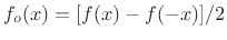 is even,
  is
odd, and
is
odd, and  .
.
.
.
.
.
.
.
.
.
.
.
.
.
.
.
.
.
.
.
.
.
.
.
.
.
.
.
.
.
.
.
- ... mapping.7.18
- Note that
memoryless nonlinearities used for distortion simulation are typically
odd functions of instantaneous amplitude, such as
 . (A good practical choice is given in
Eq.(6.19).) However, in guitar-amplifier distortion
simulation, even-order terms are considered quite important
[398].
. (A good practical choice is given in
Eq.(6.19).) However, in guitar-amplifier distortion
simulation, even-order terms are considered quite important
[398].
.
.
.
.
.
.
.
.
.
.
.
.
.
.
.
.
.
.
.
.
.
.
.
.
.
.
.
.
.
.
- ...7.19
- The convolution theorem for Fourier transforms states that
convolution in the time domain corresponds to pointwise multiplication
in the frequency domain [452]. The dual of the convolution
theorem states just the opposite: Pointwise multiplication in the time
domain corresponds to convolution in the frequency domain. Thus, if
the spectrum of
is
 , then the spectrum of
  is
is
 , where ``
 '' denotes the convolution
operation.
'' denotes the convolution
operation.
.
.
.
.
.
.
.
.
.
.
.
.
.
.
.
.
.
.
.
.
.
.
.
.
.
.
.
.
.
.
- ... spectra.7.20
- The
basilar membrane of the ear (which is rolled up inside the
snail-shaped cochlea of the ear) effectively performs a real-time
Fourier analysis which is ``felt'' by nerve cells leading to the
brain.
.
.
.
.
.
.
.
.
.
.
.
.
.
.
.
.
.
.
.
.
.
.
.
.
.
.
.
.
.
.
- ... transform|textbf,8.1
- For a short online introduction to Laplace transforms, see, e.g.,
http://ccrma.stanford.edu/~jos/filters/Laplace_Transform_Analysis.html.
.
.
.
.
.
.
.
.
.
.
.
.
.
.
.
.
.
.
.
.
.
.
.
.
.
.
.
.
.
.
- ... relation:8.2
- Of course, here we should call it the ``force
divider'' relation.
.
.
.
.
.
.
.
.
.
.
.
.
.
.
.
.
.
.
.
.
.
.
.
.
.
.
.
.
.
.
- ... mass.''8.3
- We say that the driving point of every mechanical
system must ``looks like a mass'' at sufficiently high frequency
because every mechanical system has at least some mass, and the
driving-point impedance of a mass goes to infinity with frequency.
However, in a completely detailed model, the contact force between
objects should really be the Coulombe force, which ``looks like
a spring''. In other words, mechanical interactions are ultimately
electromagnetic interactions, and it is theoretically possible for a
driving force on an atom to be so small and fast that it can vibrate
the outermost electron orbital without moving the nucleus appreciably,
thus ``looking like a spring'' in the high-frequency limit. We will
not be concerned with atomic-scale models in this book, and will
persist in treating masses and springs in idealized form.
.
.
.
.
.
.
.
.
.
.
.
.
.
.
.
.
.
.
.
.
.
.
.
.
.
.
.
.
.
.
- ...JOSFP.8.4
- Available online at
http://ccrma.stanford.edu/~jos/filters/Graphical_Amplitude_Response.html
.
.
.
.
.
.
.
.
.
.
.
.
.
.
.
.
.
.
.
.
.
.
.
.
.
.
.
.
.
.
- ....8.5
- To avoid the introduction of
half a sample of delay by the approximation, the first-order finite
difference may be defined instead as
![$ x[(n+1)T]-x[(n-1)T]/(2T)$](img1645.png) .
.
.
.
.
.
.
.
.
.
.
.
.
.
.
.
.
.
.
.
.
.
.
.
.
.
.
.
.
.
.
.
- ...JOSFP).8.6
- In
continuous time, the order is incremented once for each
independently moving mass or spring. In discrete time, the order is
increased by one when a sample of delay is added to the system
state, and the number of multiplies needed to implement a digital
simulation is bounded by twice the order plus one.
.
.
.
.
.
.
.
.
.
.
.
.
.
.
.
.
.
.
.
.
.
.
.
.
.
.
.
.
.
.
- ...JOSFP,8.7
- http://ccrma.stanford.edu/~jos/filters/State_Space_Filters.html
.
.
.
.
.
.
.
.
.
.
.
.
.
.
.
.
.
.
.
.
.
.
.
.
.
.
.
.
.
.
- ...blt).8.8
- Normally one or more output signals
 are defined as linear
combinations of the state vector
are defined as linear
combinations of the state vector
 , viz.,
 . However, we can define the state itself as the output for
now, and form any desired linear combinations separately.
. However, we can define the state itself as the output for
now, and form any desired linear combinations separately.
.
.
.
.
.
.
.
.
.
.
.
.
.
.
.
.
.
.
.
.
.
.
.
.
.
.
.
.
.
.
- ...FranklinEtAl98.9.1
- Estimating transfer functions based on
input-output measurements is called ``system identification''
[290,432]--used in advanced automatic control
applications.
.
.
.
.
.
.
.
.
.
.
.
.
.
.
.
.
.
.
.
.
.
.
.
.
.
.
.
.
.
.
- ....9.2
- For
convenience, we typically define the discrete-time counterpart of a
continuous-time function as though the sampling interval were
 .
.
.
.
.
.
.
.
.
.
.
.
.
.
.
.
.
.
.
.
.
.
.
.
.
.
.
.
.
.
.
.
- ...
response.9.3
- Frequency-domain aliasing is discussed
in [454].
.
.
.
.
.
.
.
.
.
.
.
.
.
.
.
.
.
.
.
.
.
.
.
.
.
.
.
.
.
.
- ...JOSFP:9.4
- http://ccrma.stanford.edu/~jos/filters/Partial_Fraction_Expansion.html
.
.
.
.
.
.
.
.
.
.
.
.
.
.
.
.
.
.
.
.
.
.
.
.
.
.
.
.
.
.
- ...JOSFP).9.5
- The strictly proper constraint is
natural in practice because the frequency responses of typical
real-world systems generally roll off at least -6 dB per octave.
Notice that Eq.(8.1) becomes
 as
as
 , which
is a
, which
is a  dB/octave roll off. Setting
  and
and
 yields a
  dB/octave roll-off, and so on. However, this depends
on the physical units chosen for the input and output signals of the
system. For example, consider an ideal nonzero mass driven by a
force; while the resulting velocity and displacement go to zero as
frequency goes to infinity (for any finite applied force), the
acceleration does not roll off, being proportional to applied force by
Newton's 2nd law.
dB/octave roll-off, and so on. However, this depends
on the physical units chosen for the input and output signals of the
system. For example, consider an ideal nonzero mass driven by a
force; while the resulting velocity and displacement go to zero as
frequency goes to infinity (for any finite applied force), the
acceleration does not roll off, being proportional to applied force by
Newton's 2nd law.
.
.
.
.
.
.
.
.
.
.
.
.
.
.
.
.
.
.
.
.
.
.
.
.
.
.
.
.
.
.
- ... modes.9.6
- Modal synthesis
could well be renamed ``Bernoulli synthesis,'' as Daniel Bernoulli
was quite alone in advocating the concept of seeing general
vibration as a superposition of ``simple'' sinusoidal
vibrations. This view was resisted by Euler and d'Alembert at the
time [103].
.
.
.
.
.
.
.
.
.
.
.
.
.
.
.
.
.
.
.
.
.
.
.
.
.
.
.
.
.
.
- ...JOSFP9.7
- http://ccrma.stanford.edu/~jos/filters/Modal_Representation.html
.
.
.
.
.
.
.
.
.
.
.
.
.
.
.
.
.
.
.
.
.
.
.
.
.
.
.
.
.
.
- ... response,9.8
- A
``causal frequency response''
 is the Fourier transform of
a causal impulse response
(i.e.,
is the Fourier transform of
a causal impulse response
(i.e.,  for all
).
Extensions to finitely noncausal spectra are straightforward:
Time-shift the desired impulse response to make it causal, perform
the filter design, then reverse-time-shift the filter numerator if
needed.
for all
).
Extensions to finitely noncausal spectra are straightforward:
Time-shift the desired impulse response to make it causal, perform
the filter design, then reverse-time-shift the filter numerator if
needed.
.
.
.
.
.
.
.
.
.
.
.
.
.
.
.
.
.
.
.
.
.
.
.
.
.
.
.
.
.
.
- ...9.9
- A stability margin may be specified, for example, by
requiring all poles
 to satisfy
 , where
 determines the stability margin. In particular, with
this specification on the poles, the impulse response
must
decay asymptotically at least as fast as
determines the stability margin. In particular, with
this specification on the poles, the impulse response
must
decay asymptotically at least as fast as
 [452].
.
.
.
.
.
.
.
.
.
.
.
.
.
.
.
.
.
.
.
.
.
.
.
.
.
.
.
.
.
.
- ...convex9.10
- Since convex functions bulge upward, like
the top of a circle, it makes sense to maximize them in
general. Since our error-surface formulation is always
minimized with respect to the filter parameters, we could
call it ``concave'' or ``convex from below''. In the optimization
domain, however, a ``convex'' region is one that contains all of its
chords, thus it applies to either case.
.
.
.
.
.
.
.
.
.
.
.
.
.
.
.
.
.
.
.
.
.
.
.
.
.
.
.
.
.
.
- ....9.11
-
 cannot go to infinity
since the constraint
cannot go to infinity
since the constraint
 and the stability constraint
imply that
ln
and the stability constraint
imply that
ln is zero-mean by the argument
principle [299,329].
is zero-mean by the argument
principle [299,329].
.
.
.
.
.
.
.
.
.
.
.
.
.
.
.
.
.
.
.
.
.
.
.
.
.
.
.
.
.
.
- ... Octave.9.12
- Octave's remez
function and Matlab's firpm function (Signal Processing
Toolbox) have a special mode for designing FIR differentiators that
are optimal in the Chebeshev sense, while invfreqz
minimizes equation error, which is arguably not as good. We focus
on invfreqz in this chapter because it offers the level
of generality needed for fitting digital filters to arbitrary
measured frequency responses.
.
.
.
.
.
.
.
.
.
.
.
.
.
.
.
.
.
.
.
.
.
.
.
.
.
.
.
.
.
.
- ...9.13
- When working with invfreqz, it is often helpful to
multiply the desired spectrum by a linear phase term [452]
corresponding to an added delay in the impulse response [432].
The filter designed by invfreqz will typically be stable if
sufficient delay is added to the desired frequency response in this
way. Thus, if a filter designed by invfreqz is found to be
unstable, multiply the desired frequency response by a steeper
negative-slope linear-phase term and repeat the design.
.
.
.
.
.
.
.
.
.
.
.
.
.
.
.
.
.
.
.
.
.
.
.
.
.
.
.
.
.
.
- ... data.9.14
- The number of poles and zeros needed for a
reasonable fit were determined empirically. No zeros gives a poor
overall match, and only two poles yields a significantly less sharp
resonant peak.
.
.
.
.
.
.
.
.
.
.
.
.
.
.
.
.
.
.
.
.
.
.
.
.
.
.
.
.
.
.
- ...
responses.9.15
- Ideally, they are also constrained to produce
stable filters as well, but invfreqz does not offer
a stability constraint, and so stability should be checked whenever
specifying one or more poles.
.
.
.
.
.
.
.
.
.
.
.
.
.
.
.
.
.
.
.
.
.
.
.
.
.
.
.
.
.
.
- ...JOSFP.9.16
- https://ccrma.stanford.edu/~jos/filters/Creating_Minimum_Phase_Filters.html
.
.
.
.
.
.
.
.
.
.
.
.
.
.
.
.
.
.
.
.
.
.
.
.
.
.
.
.
.
.
- ...SB.9.17
- SynthBuilder is now a proprietary
in-house tool at Analog Devices, Inc. See [86] for a
description of the STK software prototyping environment that many of
us use today. In particular, the Mandolin.cpp patch in the
STK distribution is based on commuted synthesis. Some of us are also
using the STK package in conjunction with pd [358] in
order to obtain drag-and-drop graphical patch construction and a
large library of MIDI processing tools.
.
.
.
.
.
.
.
.
.
.
.
.
.
.
.
.
.
.
.
.
.
.
.
.
.
.
.
.
.
.
- ...SmithCommutedFromPASP,MattiGuitar,MattiAndSmith96.9.18
- Extracts of
this material were published previously in [230].
.
.
.
.
.
.
.
.
.
.
.
.
.
.
.
.
.
.
.
.
.
.
.
.
.
.
.
.
.
.
- ... volume.9.19
- These remarks apply to playback of the
excitation only. The string provides further filtering which could be
taken into account. However, to a first approximation, the string
filtering is like a ``sampling'' of the excitation spectrum, with a
gentle roll-off at high frequencies due to the lowpass loop
filtering. Also, the string is a highly variable filter with many
settings. It is therefore reasonable to ignore the string filtering
when determining an optimal preemphasis for excitation-table
quantization.
.
.
.
.
.
.
.
.
.
.
.
.
.
.
.
.
.
.
.
.
.
.
.
.
.
.
.
.
.
.
- ...allpass1phaser.9.20
- This is the
basic architecture of the MXR phase shifter as well as the
Univibe used by Jimi Hendrix [243], and described in
detail at (http://www.geofex.com/Article_Folders/univibe/uvfrindx.htm).
.
.
.
.
.
.
.
.
.
.
.
.
.
.
.
.
.
.
.
.
.
.
.
.
.
.
.
.
.
.
- ...
filters,9.21
- Moog has built a 12-stage phaser of this type
[59] and up to 20 stages (10 notches) have been noted
[244].
.
.
.
.
.
.
.
.
.
.
.
.
.
.
.
.
.
.
.
.
.
.
.
.
.
.
.
.
.
.
- ...JOSFP9.22
- Available online at
http://ccrma.stanford.edu/~jos/filters/Analog_Allpass_Filters.html
.
.
.
.
.
.
.
.
.
.
.
.
.
.
.
.
.
.
.
.
.
.
.
.
.
.
.
.
.
.
- ...9.23
- Saying that the frequency
 is the
break frequency for the one-pole term
is the
break frequency for the one-pole term
 is
terminology from classical control theory.
Below the break frequency,
is
terminology from classical control theory.
Below the break frequency,
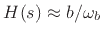 , and above,
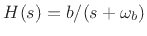 . On a log-log plot, the amplitude response
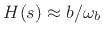 may be approximated by a slope-zero line at height
 from dc to
, followed by an
intersecting line with negative slope of 20 dB per decade for all
higher frequencies. At the break frequency, the true gain is down 3 dB
from
from dc to
, followed by an
intersecting line with negative slope of 20 dB per decade for all
higher frequencies. At the break frequency, the true gain is down 3 dB
from  , but far away from the break frequency, the
piecewise-linear approximation is very accurate. Such a plot of the
log-frequency-response versus log-frequency (the real part being log-magnitude
and the imaginary part being phase, plotted separately)
is called a Bode plot. Bode
plots are covered in any introductory course on control systems design
(also called the design of ``servomechanisms''), and see also the Wikipedia
page for ``Bode plot.''
, but far away from the break frequency, the
piecewise-linear approximation is very accurate. Such a plot of the
log-frequency-response versus log-frequency (the real part being log-magnitude
and the imaginary part being phase, plotted separately)
is called a Bode plot. Bode
plots are covered in any introductory course on control systems design
(also called the design of ``servomechanisms''), and see also the Wikipedia
page for ``Bode plot.''
.
.
.
.
.
.
.
.
.
.
.
.
.
.
.
.
.
.
.
.
.
.
.
.
.
.
.
.
.
.
- ... response:10.1
- The
corresponding impulse response is
![$ h=[\ldots,0,{\hat g}(1),{\hat g}(0),{\hat g}(1),0,\ldots]$](img1955.png) , where
, where
 occurs at
time 0, and the transfer function is
occurs at
time 0, and the transfer function is
![$ {\hat G}(z) = {\hat g}(0) +
{\hat g}(1)[z+z^{-1}]$](img1957.png) . In practice, this filter is typically
implemented in causal form, i.e.,
. In practice, this filter is typically
implemented in causal form, i.e.,
![$ h = [{\hat g}(1),{\hat g}(0),{\hat g}(1),0,\ldots]$](img1958.png) starting at time 0, and one sample of delay is subtracted from a
delay-line preceding or following the filter.
starting at time 0, and one sample of delay is subtracted from a
delay-line preceding or following the filter.
.
.
.
.
.
.
.
.
.
.
.
.
.
.
.
.
.
.
.
.
.
.
.
.
.
.
.
.
.
.
- ...
law,10.2
- A function
is said to be odd if
 .
.
.
.
.
.
.
.
.
.
.
.
.
.
.
.
.
.
.
.
.
.
.
.
.
.
.
.
.
.
.
.
- ... function:10.3
- See
http://www.trueaudio.com/at_eetjlm.htm
for further discussion.
.
.
.
.
.
.
.
.
.
.
.
.
.
.
.
.
.
.
.
.
.
.
.
.
.
.
.
.
.
.
- ... output.10.4
- So-called
``electric-acoustic'' guitars, such as the Godin electric-acoustic,
use piezoelectric crystals in the bridge to measure string force at
the string endpoint. Electric violins, such as the Zeta Violin,
typically use this approach as well.
.
.
.
.
.
.
.
.
.
.
.
.
.
.
.
.
.
.
.
.
.
.
.
.
.
.
.
.
.
.
- ...
measurements.10.5
- The matlab function cohere() can be
used to compute the coherence function between two signals across
multiple physical measurements (one per non-overlapping frame).
.
.
.
.
.
.
.
.
.
.
.
.
.
.
.
.
.
.
.
.
.
.
.
.
.
.
.
.
.
.
- ... phase.10.6
- Zero-phase filters can normally be
implemented in practice because there are pure delay lines preceding and
following the reflectance filter, and taps can be introduced in the
delay-line preceding the reflectance to implement noncausal terms in the
impulse response.
.
.
.
.
.
.
.
.
.
.
.
.
.
.
.
.
.
.
.
.
.
.
.
.
.
.
.
.
.
.
- ....10.7
- To
prove this, note that the roots of
 are the reciprocals of the
roots of
are the reciprocals of the
roots of  , since the conformal map
 exchanges
interior of the unit circle with the exterior of the unit circle.
exchanges
interior of the unit circle with the exterior of the unit circle.
.
.
.
.
.
.
.
.
.
.
.
.
.
.
.
.
.
.
.
.
.
.
.
.
.
.
.
.
.
.
- ... below.10.8
- In
particular, as illustrated in Fig.9.14 below, we can
formulate the initial mass momentum as being supplied by an external
impulsive force at time zero.
.
.
.
.
.
.
.
.
.
.
.
.
.
.
.
.
.
.
.
.
.
.
.
.
.
.
.
.
.
.
- ... transform10.9
- http://ccrma.stanford.edu/~jos/filters/Introduction_Laplace_Transform_Analysis.html
.
.
.
.
.
.
.
.
.
.
.
.
.
.
.
.
.
.
.
.
.
.
.
.
.
.
.
.
.
.
- ...JOSFP.10.10
- http://ccrma.stanford.edu/~jos/filters/Differentiation.html
.
.
.
.
.
.
.
.
.
.
.
.
.
.
.
.
.
.
.
.
.
.
.
.
.
.
.
.
.
.
- ... function,10.11
 for
for
 and 1 for
 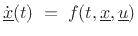 .
.
.
.
.
.
.
.
.
.
.
.
.
.
.
.
.
.
.
.
.
.
.
.
.
.
.
.
.
.
.
.
- ...10.12
- In acoustic tubes, it is the
longitudinal-velocity wave variable that changes sign when the
direction of propagation is changed, because the air particles then
move in the opposite direction along the tube axis
. The
pressure, on the other hand, being a scalar field, does not
fundamentally change sign when the propagation direction toggles.
.
.
.
.
.
.
.
.
.
.
.
.
.
.
.
.
.
.
.
.
.
.
.
.
.
.
.
.
.
.
- ... string.10.13
- Since we
are in continuous time, a notation more consistent with
Chapter 6 would be
 and
and
 , for
, for  , as we reserved the
  superscripts
for the discrete-time case in that chapter. Notation has thus been
changed for this example.
superscripts
for the discrete-time case in that chapter. Notation has thus been
changed for this example.
.
.
.
.
.
.
.
.
.
.
.
.
.
.
.
.
.
.
.
.
.
.
.
.
.
.
.
.
.
.
- ...Suzuki,Boutillon88,HallAndAskenfelt88,ChaigneAndAskenfeltII,BorinAndDePoli,Stulov95,GiordanoAndMillis01.10.14
- http://www.acs.psu.edu/drussell/Piano/NonlinearHammer.html
.
.
.
.
.
.
.
.
.
.
.
.
.
.
.
.
.
.
.
.
.
.
.
.
.
.
.
.
.
.
- ...
model).10.15
- See, e.g.,
[350] for a more elaborate model in which release
is calculated from the computed geometry of the plectrum.
.
.
.
.
.
.
.
.
.
.
.
.
.
.
.
.
.
.
.
.
.
.
.
.
.
.
.
.
.
.
- ... that.10.16
- Of course, a
truly complete plucking model would allow the plectrum to move in 3D
space, at least within a plucking plane, and the collision detection
would determine when the string (a point whirling about in the
plucking plane) intersects the plectrum.
.
.
.
.
.
.
.
.
.
.
.
.
.
.
.
.
.
.
.
.
.
.
.
.
.
.
.
.
.
.
- ... D.10.17
- The
PC88 stretching begins in the fourth octave, while the measured
Steinway stretching is greatest in the first octave (reaching nearly
-20 cents relative to ``nominal tuning'' for the first note A0) and
picking up again, going sharp, in the sixth octave. See
http://www.precisionstrobe.com/apps/stretchdata/stretchdata.html
for the measured curves.
.
.
.
.
.
.
.
.
.
.
.
.
.
.
.
.
.
.
.
.
.
.
.
.
.
.
.
.
.
.
- ... order,10.18
- It is
valid to neglect the reed mass when the first reed resonance is well
above the fundamental frequency of the played note, as is normally
the case.
.
.
.
.
.
.
.
.
.
.
.
.
.
.
.
.
.
.
.
.
.
.
.
.
.
.
.
.
.
.
- ...
closure.10.19
- For operation in fixed-point DSP chips, the
independent variable
 is generally confined to the interval
  . Note that having the
table go all the way to zero at the maximum negative pressure
. Note that having the
table go all the way to zero at the maximum negative pressure
 is not physically reasonable (0.8 would be more reasonable), but it has the
practical benefit that when the lookup-table input signal is about to clip,
the reflection coefficient goes to zero, thereby opening the feedback
loop.
is not physically reasonable (0.8 would be more reasonable), but it has the
practical benefit that when the lookup-table input signal is about to clip,
the reflection coefficient goes to zero, thereby opening the feedback
loop.
.
.
.
.
.
.
.
.
.
.
.
.
.
.
.
.
.
.
.
.
.
.
.
.
.
.
.
.
.
.
- ... motion|textbf10.20
- https://ccrma.stanford.edu/realsimple/travelingwaves/Helmholtz_Motion.html
.
.
.
.
.
.
.
.
.
.
.
.
.
.
.
.
.
.
.
.
.
.
.
.
.
.
.
.
.
.
- ...exponentially10.21
- If the flare of the bell is expressed as
 , where
 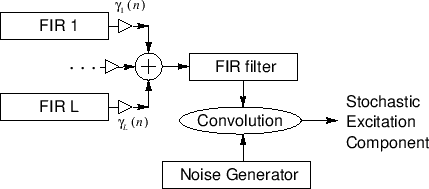 denotes the horn radius at
position
along the bore axis, then
denotes the horn radius at
position
along the bore axis, then  is called the
flare constant of the bell.
is called the
flare constant of the bell.
.
.
.
.
.
.
.
.
.
.
.
.
.
.
.
.
.
.
.
.
.
.
.
.
.
.
.
.
.
.
- ... pressure10.22
- As always
in this book, by ``air pressure'' we mean the excess air
pressure above ambient air pressure. In the case of brass
instruments, excess air pressure is created by the muscles of the
lungs.
.
.
.
.
.
.
.
.
.
.
.
.
.
.
.
.
.
.
.
.
.
.
.
.
.
.
.
.
.
.
- ... mouthpiece.10.23
- When
the kinetic energy of a jet is converted back into air pressure, this
is called pressure recovery. We assume, following
[98] and others, that pressure recovery does not occur
in this model. Instead, the kinetic energy of the jet is assumed to
be dissipated in the form of turbulence (vortices and ultimately
heat). Note that air flow is therefore assumed inviscid within the
mouth and between the lips, but viscous around the jet in the
mouthpiece.
.
.
.
.
.
.
.
.
.
.
.
.
.
.
.
.
.
.
.
.
.
.
.
.
.
.
.
.
.
.
- ...Putland.10.24
- For velocity waves, the flare may be
hyperbolic [50].
.
.
.
.
.
.
.
.
.
.
.
.
.
.
.
.
.
.
.
.
.
.
.
.
.
.
.
.
.
.
- ...dAlembert,Darrigol07.A.1
- For a short biography of d'Alembert, see
http:
//www-groups.dcs.st-and.ac.uk/~history/Mathematicians/D'Alembert.html
.
.
.
.
.
.
.
.
.
.
.
.
.
.
.
.
.
.
.
.
.
.
.
.
.
.
.
.
.
.
- ... (1685-1731)A.2
- http:
//<ibidem>/Taylor.html
.
.
.
.
.
.
.
.
.
.
.
.
.
.
.
.
.
.
.
.
.
.
.
.
.
.
.
.
.
.
- ... (1707-1783)A.3
- http:
//<ibidem>/Euler.html
.
.
.
.
.
.
.
.
.
.
.
.
.
.
.
.
.
.
.
.
.
.
.
.
.
.
.
.
.
.
- ...
eyeglasses.A.4
- http://www.mathphysics.com/pde/history.html
.
.
.
.
.
.
.
.
.
.
.
.
.
.
.
.
.
.
.
.
.
.
.
.
.
.
.
.
.
.
- ...Darrigol07.A.5
- http:
//www.stetson.edu/~efriedma/periodictable/html/B.html
.
.
.
.
.
.
.
.
.
.
.
.
.
.
.
.
.
.
.
.
.
.
.
.
.
.
.
.
.
.
- ...ZadehAndDesoer,Kailath80,Depalle.A.6
- http://ccrma.stanford.edu/~jos/PianoString/
.
.
.
.
.
.
.
.
.
.
.
.
.
.
.
.
.
.
.
.
.
.
.
.
.
.
.
.
.
.
- ...strain.A.7
- http://www.efunda.com/formulae/solid_mechanics/mat_mechanics/hooke.cfm
.
.
.
.
.
.
.
.
.
.
.
.
.
.
.
.
.
.
.
.
.
.
.
.
.
.
.
.
.
.
- ...
public.A.8
- http:
//cnx.rice.edu/content/m0050/latest/
.
.
.
.
.
.
.
.
.
.
.
.
.
.
.
.
.
.
.
.
.
.
.
.
.
.
.
.
.
.
- ...FettweisMain.A.9
- Derivation:
http://ccrma.stanford.edu/~jos/pasp/Wave_Digital_Filters.html
.
.
.
.
.
.
.
.
.
.
.
.
.
.
.
.
.
.
.
.
.
.
.
.
.
.
.
.
.
.
- ...
Belevitch.A.10
- http://www.ieee.org/organizations/history_center/oral_histories/transcripts/fettweis.html
.
.
.
.
.
.
.
.
.
.
.
.
.
.
.
.
.
.
.
.
.
.
.
.
.
.
.
.
.
.
- ...Flanagan72,FlanaganAndRabinerEds,RabinerAndSchafer10,SchaferAndMarkel79,OShaughnessy87,DPH01,Keller94.A.11
- The
overview [309] of early speech production models is
freely available online, thanks to the Smithsonian Speech Synthesis
History Project.
.
.
.
.
.
.
.
.
.
.
.
.
.
.
.
.
.
.
.
.
.
.
.
.
.
.
.
.
.
.
- ... formulation.A.12
- http:
en.wikipedia.org/wiki/Oliver_Heaviside
.
.
.
.
.
.
.
.
.
.
.
.
.
.
.
.
.
.
.
.
.
.
.
.
.
.
.
.
.
.
- ... phenomenon.A.13
- http:www.microwaves101.com/encyclopedia/history.cfm
.
.
.
.
.
.
.
.
.
.
.
.
.
.
.
.
.
.
.
.
.
.
.
.
.
.
.
.
.
.
- ...A.14
- Scattering
theory:
http://ccrma.stanford.edu/~jos/pasp/Scattering_Impedance_Changes.html
.
.
.
.
.
.
.
.
.
.
.
.
.
.
.
.
.
.
.
.
.
.
.
.
.
.
.
.
.
.
- ... method.A.15
- ``Bicycle Built for
Two'' by Kelly, Lochbaum, and Matthews,
1961:
http://ccrma.stanford.edu/~jos/wav/daisy-klm.wav
.
.
.
.
.
.
.
.
.
.
.
.
.
.
.
.
.
.
.
.
.
.
.
.
.
.
.
.
.
.
- ... completion.A.16
- http://www.bell-labs.com/news/1997/march/5/2.html
.
.
.
.
.
.
.
.
.
.
.
.
.
.
.
.
.
.
.
.
.
.
.
.
.
.
.
.
.
.
- ...PRCT.A.17
- http:
www.cs.princeton.edu/~prc/SingingSynth.html (includes sound
examples)
.
.
.
.
.
.
.
.
.
.
.
.
.
.
.
.
.
.
.
.
.
.
.
.
.
.
.
.
.
.
- ...PainterAndSpanias2000.A.18
- In particular, CELP is used in the
free, open-source speech codec called Speex
(http://www.speex.org).
.
.
.
.
.
.
.
.
.
.
.
.
.
.
.
.
.
.
.
.
.
.
.
.
.
.
.
.
.
.
- ...SchellengA,SchellengB,CremerC.A.19
- http://www.zainea.com/Oscilationsofbowedstring.htm
.
.
.
.
.
.
.
.
.
.
.
.
.
.
.
.
.
.
.
.
.
.
.
.
.
.
.
.
.
.
- ...
excitation.A.20
- The Karplus-Strong U.S. patent 4,649,783A,
``Wavetable-modification instrument and method for generating musical
sound,'' has the following abstract: A musical instrument employing
probabilistic wavetable-modification method of producing musical
sound. A randomly initialized wavetable which is periodically accessed
to provide an output signal which determines the musical sound. The
output signal from the wavetable is probabilistically modified and
stored back into the wavetable as modified data. The modified data,
after a delay, is accessed from the wavetable and thereby becomes a
new output signal. This process is periodically repeated whereby each
new output signal is stored (after possibly being modified) back into
the wavetable to produce rich and natural musical sound.
.
.
.
.
.
.
.
.
.
.
.
.
.
.
.
.
.
.
.
.
.
.
.
.
.
.
.
.
.
.
- ...
simpleB.1
- While this formula seems fairly simple now, in
Newton's day, it was necessary to invent calculus before it
could be stated in this way.
.
.
.
.
.
.
.
.
.
.
.
.
.
.
.
.
.
.
.
.
.
.
.
.
.
.
.
.
.
.
- ... constant.B.2
- The gravitation constant is given in
International Standard Units (``SI units'') by
where the following physical units abbreviations are used:
The physical units for newtons follow from Newton's second law of
motion  , and the physical units for
  follow immediately from
Eq.(B.2).
follow immediately from
Eq.(B.2).
.
.
.
.
.
.
.
.
.
.
.
.
.
.
.
.
.
.
.
.
.
.
.
.
.
.
.
.
.
.
- ...force|textbf.B.3
- From
a modern point of view, all forces are ``mediated'' by some particle,
and there are only four basic forces: The electromagnetic force
is mediated by the photon, the
strong nuclear force is mediated
by the gluon, the weak nuclear force is mediated by the
and
 bosons, and gravity is thought to be mediated by
the graviton, although gravity is not yet incorporated into the
Standard Model
of theoretical physics. Only the electromagnetic
and gravitational forces are encountered in everyday life, since the
strong and weak nuclear forces decay exponentially on the scale of an
atomic nucleus.
bosons, and gravity is thought to be mediated by
the graviton, although gravity is not yet incorporated into the
Standard Model
of theoretical physics. Only the electromagnetic
and gravitational forces are encountered in everyday life, since the
strong and weak nuclear forces decay exponentially on the scale of an
atomic nucleus.
.
.
.
.
.
.
.
.
.
.
.
.
.
.
.
.
.
.
.
.
.
.
.
.
.
.
.
.
.
.
- ... force.B.4
- In this example, the
mass-spring system is in
equilibrium (not moving), so all forces in the system must sum
to zero. Equilibrium also must hold if the whole system is traveling
with a constant velocity; in other words, it is the lack of
relative motion that matters.
.
.
.
.
.
.
.
.
.
.
.
.
.
.
.
.
.
.
.
.
.
.
.
.
.
.
.
.
.
.
- ... displacements.B.5
- To show
this quantitatively, consider two electrons, each having electric
charge
 , separated by
  meters. Then the Coulomb force between
the electrons is proportional to
meters. Then the Coulomb force between
the electrons is proportional to  . Adding a small
perturbation
. Adding a small
perturbation  to
yields a new force proportional to
to
yields a new force proportional to
where we used the binomial expansion to obtain the
approximation. (The notation
 means ``terms order
of
means ``terms order
of
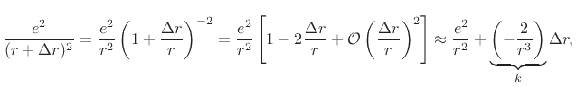 '', and such terms approach zero as fast as
approaches zero.) Thus, the effective spring constant
connecting the two electrons is
'', and such terms approach zero as fast as
approaches zero.) Thus, the effective spring constant
connecting the two electrons is  , when
 .
.
.
.
.
.
.
.
.
.
.
.
.
.
.
.
.
.
.
.
.
.
.
.
.
.
.
.
.
.
.
.
- ...
yieldingB.6
- A more formal methodology for arriving
at differential equations by applying Newton's law and Hooke's law is
described in Appendix F. In the present example, consideration of the
underlying physics should convince you that the signs in Eq.(B.4)
are correct. For example, when
is positive, the spring must push
the mass back to the left. Therefore,
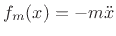 means the mass
will be accelerated to the left.
means the mass
will be accelerated to the left.
.
.
.
.
.
.
.
.
.
.
.
.
.
.
.
.
.
.
.
.
.
.
.
.
.
.
.
.
.
.
- ...
time:B.7
- See, e.g.,
[452, p. 313-316] for a derivation, and Appendix F,
specifically §F.3.6, for related analysis.
.
.
.
.
.
.
.
.
.
.
.
.
.
.
.
.
.
.
.
.
.
.
.
.
.
.
.
.
.
.
- ...
object.B.8
- In SI units, work is in units called
joules (abbreviated J
).
Thus, joules are newtons times meters.
Power in watts is defined as joules per second.
One joule is the energy dissipated in one second
by an electric current of one ampere (coulomb per second) through a
resistance of one ohm. For a list of physical units and their abbreviations,
see, for example, http://physics.nist.gov/cuu/Units/units.html.
.
.
.
.
.
.
.
.
.
.
.
.
.
.
.
.
.
.
.
.
.
.
.
.
.
.
.
.
.
.
- ... considered.B.9
- Ok, there does exist energy
fluctuation on the scale of ``Heisenberg uncertainty''. That is, it
is possible to have a violation in energy conservation by an amount
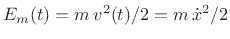 over a time duration
  , provided
 is sufficiently small (on the order of Planck's constant
  ).
This can be considered a form of the Heisenberg uncertainty principle.
).
This can be considered a form of the Heisenberg uncertainty principle.
.
.
.
.
.
.
.
.
.
.
.
.
.
.
.
.
.
.
.
.
.
.
.
.
.
.
.
.
.
.
- ...
general.B.10
- Conservation of energy and momentum are unified in
what is called the ``four-momentum'' of spacetime,
![$ P=[E/c,p_x,p_y,p_z]$](img2699.png) ,
often used in special relativity calculations (see,
e.g., http://en.wikipedia.org/wiki/Four-momentum). Thus,
energy (divided by the speed of light
) is just the 0th component
of the four-momentum.
,
often used in special relativity calculations (see,
e.g., http://en.wikipedia.org/wiki/Four-momentum). Thus,
energy (divided by the speed of light
) is just the 0th component
of the four-momentum.
.
.
.
.
.
.
.
.
.
.
.
.
.
.
.
.
.
.
.
.
.
.
.
.
.
.
.
.
.
.
- ... space.B.11
- Additionally, mechanics problems are
formulated using the principle of least action, in which the
action is defined as the time integral of the Lagrangian
(usually the kinetic energy minus potential energy). Equations of
motion, including Newton's second law, are obtained by finding the
path which minimizes this action integral. The two main resulting
formulations for the equations of motion (in addition to Newton's
formulation) are called the Lagrangian and Hamiltonian
formulations, and they generalize more cleanly to constrained motion,
more general phase-space coordinate systems, relativistic
invariance, and problems in quantum mechanics. Another nice
implication of the principle of least action is that the conservation
of energy follows from homogeneity of time, and conservation of
momentum from isotropy of space [272]. We will
be fine with the classical Newtonian formulation here.
.
.
.
.
.
.
.
.
.
.
.
.
.
.
.
.
.
.
.
.
.
.
.
.
.
.
.
.
.
.
- ... points:B.12
- We denote by
 the set of all points in 3D Euclidean space. Thus
 has three coordinates, usually denoted
,
, and
, or (as we
will use below),
has three coordinates, usually denoted
,
, and
, or (as we
will use below),  ,
,  , and
, and  , all real scalars
(
, all real scalars
(
 ).
).
.
.
.
.
.
.
.
.
.
.
.
.
.
.
.
.
.
.
.
.
.
.
.
.
.
.
.
.
.
.
- ...
rotatingB.13
- We are generally concerned with the rotation of a
rigid body about some axis passing through its center of
mass. Therefore, we will not distinguish between ``rotating,'' as
the earth does to produce night and day, and ``revolving,'' as the
earth does around the sun to produce the seasons. Thus, the
individual mass particles of a rotating rigid body will be said to
rotate about the axis of rotation, even though ``revolve''
might win more points on a middle-school exam.
.
.
.
.
.
.
.
.
.
.
.
.
.
.
.
.
.
.
.
.
.
.
.
.
.
.
.
.
.
.
- ...,B.14
- To create a rigid collection of point masses,
we can imagine them to be interconnected by ``massless rigid rods''
or, equivalently, ideal springs having infinite stiffness.
.
.
.
.
.
.
.
.
.
.
.
.
.
.
.
.
.
.
.
.
.
.
.
.
.
.
.
.
.
.
- ...
densityB.15
- We let
be a force density (a linear,
spatial, force density, in newtons per meter) in order that it can
be impulsive along
as well as
. We could have instead chosen
a force
 applied at a particular point
.
applied at a particular point
.
.
.
.
.
.
.
.
.
.
.
.
.
.
.
.
.
.
.
.
.
.
.
.
.
.
.
.
.
.
.
- ... frame|textbfB.16
- At this stage, a
better name for ``body-fixed frame'' would be center-of-mass
frame. However, later on, we will see that not only do we need
to follow the center-of-mass with the origin of our body-fixed
frame, but its coordinate axes will also need to remain pointing in
the so-called principal directions (defined in
§B.4.16).
.
.
.
.
.
.
.
.
.
.
.
.
.
.
.
.
.
.
.
.
.
.
.
.
.
.
.
.
.
.
- ... time.B.17
- There is no problem with
conservation of momentum here. We will see in §B.4.13
that, for a rotating mass
 at radius
, the angular momentum
at radius
, the angular momentum
 is always
times the
instantaneous linear momentum
is always
times the
instantaneous linear momentum  . Thus, in our problem,
converting angular momentum
. Thus, in our problem,
converting angular momentum 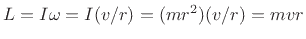 to linear momentum
  (in
the body-fixed frame) verifies conservation of momentum when we add
it to the linear momentum of the center of mass, which was also
found to be
(in
the body-fixed frame) verifies conservation of momentum when we add
it to the linear momentum of the center of mass, which was also
found to be  . In other words, the total momentum is still
  ,
as initially delivered to the system.
,
as initially delivered to the system.
.
.
.
.
.
.
.
.
.
.
.
.
.
.
.
.
.
.
.
.
.
.
.
.
.
.
.
.
.
.
- ... vector.B.18
- Another analogy is the right-hand
screw, in which the screw drives in the direction of the vector
when it is turned clockwise from behind, as is standard.
.
.
.
.
.
.
.
.
.
.
.
.
.
.
.
.
.
.
.
.
.
.
.
.
.
.
.
.
.
.
- ...matrix!determinant|textbf:B.19
- http://mathworld.wolfram.com/CrossProduct.html
.
.
.
.
.
.
.
.
.
.
.
.
.
.
.
.
.
.
.
.
.
.
.
.
.
.
.
.
.
.
- ... rule|textbf.B.20
- Rotate
to
by
``pushing'' with the fingers of the right hand, taking the smallest
angle possible, and your thumb points in the positive direction for
 .
.
.
.
.
.
.
.
.
.
.
.
.
.
.
.
.
.
.
.
.
.
.
.
.
.
.
.
.
.
.
.
- ... them:B.21
- We are using ``
 ''
(optionally, when it looks better) to denote scalar
multiplication here, while in vector calculus,
''
(optionally, when it looks better) to denote scalar
multiplication here, while in vector calculus,
 would normally denote a dot product of the two vectors
and
, but we are writing the dot product as
would normally denote a dot product of the two vectors
and
, but we are writing the dot product as
 . (We could also use the ``inner-product''
notation
. (We could also use the ``inner-product''
notation
 for real vectors [454].)
We could say that ``
'' means ordinary multiplication when
appearing between two scalars, and it means the dot product when
used between two vectors. Between two matrices it would of course
mean matrix multiplication.
for real vectors [454].)
We could say that ``
'' means ordinary multiplication when
appearing between two scalars, and it means the dot product when
used between two vectors. Between two matrices it would of course
mean matrix multiplication.
.
.
.
.
.
.
.
.
.
.
.
.
.
.
.
.
.
.
.
.
.
.
.
.
.
.
.
.
.
.
- ...conserved.B.22
- Angular momentum is also conserved on the
smallest scales, such as orbital angular momentum and the
spin of fundamental particles such as an electron. Thus,
conservation of angular momentum is a fundamental invariant in
physics, along with conservation of energy and conservation of
linear momentum. Since we live in 3D, that makes seven
conserved quantities pertaining to motion of a mass through empty
space: its kinetic energy, the three components of the linear
momentum of its center of mass, and the three components of its
angular momentum if it is rotating about its center of mass.
.
.
.
.
.
.
.
.
.
.
.
.
.
.
.
.
.
.
.
.
.
.
.
.
.
.
.
.
.
.
- ... identityB.23
- In maxima, one can
verify this identity with the following input (the output of which
is
![$ [0,0,0]$](img2870.png) ):
):
load(vect);
A:[A1,A2,A3]; B:[B1,B2,B3]; C:[C1,C2,C3];
expand(express((A ~ (B ~ C)) - (B * (C . A) - C * (A . B))));
Note that the cross-product is called the wedge product in
maxima, and is denoted by a tilde (~).
.
.
.
.
.
.
.
.
.
.
.
.
.
.
.
.
.
.
.
.
.
.
.
.
.
.
.
.
.
.
- ... balanced|textbf.B.24
-
http://www.ph.man.ac.uk/~mikeb/lecture/pc167/rigidbody/principal.html
.
.
.
.
.
.
.
.
.
.
.
.
.
.
.
.
.
.
.
.
.
.
.
.
.
.
.
.
.
.
- ...JOSFP,B.25
- https://ccrma.stanford.edu/~jos/filters/Diagonalizing_State_Space_Model.html
.
.
.
.
.
.
.
.
.
.
.
.
.
.
.
.
.
.
.
.
.
.
.
.
.
.
.
.
.
.
- ...
revolution|textbf.B.26
- http://mathworld.wolfram.com/SolidofRevolution.html
.
.
.
.
.
.
.
.
.
.
.
.
.
.
.
.
.
.
.
.
.
.
.
.
.
.
.
.
.
.
- ... vector:B.27
- Here we are using '
' to
denote the ``dot product'' (or scalar product, or inner product),
since that is the traditional notation in physics. Since it appears
between two vectors, this usage is unambiguous. Thus, we have the
following equivalent notations:
 .
.
.
.
.
.
.
.
.
.
.
.
.
.
.
.
.
.
.
.
.
.
.
.
.
.
.
.
.
.
.
.
- ... frameB.28
- An inertial frame means an
unaccelerated frame. That is, the coordinate system is not
spinning or accelerated in any way. (Even gravity is neglected.)
.
.
.
.
.
.
.
.
.
.
.
.
.
.
.
.
.
.
.
.
.
.
.
.
.
.
.
.
.
.
- ... equations:B.29
- http://www.physicsforums.com/library.php?do=view_item&itemid=182
.
.
.
.
.
.
.
.
.
.
.
.
.
.
.
.
.
.
.
.
.
.
.
.
.
.
.
.
.
.
- ... potential:B.30
- This was first pointed out
by Rayleigh
[352, p. 39].
.
.
.
.
.
.
.
.
.
.
.
.
.
.
.
.
.
.
.
.
.
.
.
.
.
.
.
.
.
.
- ... gas|textbf.B.31
- Air has been measured to contain 75.54% nitrogen and
23.10% oxygen, both of which are diatomic gases. Thus, dry air is
about 99% diatomic.
.
.
.
.
.
.
.
.
.
.
.
.
.
.
.
.
.
.
.
.
.
.
.
.
.
.
.
.
.
.
- ...Fitzpatrick.B.32
- This is a
rare example in which quantum mechanics must be considered in an
acoustic calculation!
.
.
.
.
.
.
.
.
.
.
.
.
.
.
.
.
.
.
.
.
.
.
.
.
.
.
.
.
.
.
- ...B.33
-
http://www.grc.nasa.gov/WWW/K-12/airplane/sound.html
.
.
.
.
.
.
.
.
.
.
.
.
.
.
.
.
.
.
.
.
.
.
.
.
.
.
.
.
.
.
- ... air.B.34
- Air is predominately diatomic due to
nitrogen (
 , 78%) and oxygen (
 , 21%) comprising 99% of
the Earth's atmosphere.
, 21%) comprising 99% of
the Earth's atmosphere.
.
.
.
.
.
.
.
.
.
.
.
.
.
.
.
.
.
.
.
.
.
.
.
.
.
.
.
.
.
.
- ...MDFT.B.35
- http://ccrma.stanford.edu/~jos/mdft/Projection.html
.
.
.
.
.
.
.
.
.
.
.
.
.
.
.
.
.
.
.
.
.
.
.
.
.
.
.
.
.
.
- ... relation.B.36
- Do not be misled by the name
``dispersion relation'' into thinking that wave propagation is
dispersive in this case--it is not. Dispersion occurs when
 changes as a function of frequency; here it is a
constant. Thus, the dispersion relation implies wave propagation
dispersion when
is a nonlinear function of
changes as a function of frequency; here it is a
constant. Thus, the dispersion relation implies wave propagation
dispersion when
is a nonlinear function of  .
.
.
.
.
.
.
.
.
.
.
.
.
.
.
.
.
.
.
.
.
.
.
.
.
.
.
.
.
.
.
.
- ...C.1
- Any function of
 , where
denotes time and
denotes
position along a ``waveshape'', may be interpreted as a fixed
waveshape traveling to the right (positive
direction), with
speed
. Similarly, any function of
, where
denotes time and
denotes
position along a ``waveshape'', may be interpreted as a fixed
waveshape traveling to the right (positive
direction), with
speed
. Similarly, any function of  may be seen as a
waveshape traveling to the left (negative
direction) at
speed
meters per second. In both cases,
denotes a position
along the waveshape, and
denotes time. For any fixed
, a
``snapshot'' of the waveshape may be seen by evaluating along
.
may be seen as a
waveshape traveling to the left (negative
direction) at
speed
meters per second. In both cases,
denotes a position
along the waveshape, and
denotes time. For any fixed
, a
``snapshot'' of the waveshape may be seen by evaluating along
.
.
.
.
.
.
.
.
.
.
.
.
.
.
.
.
.
.
.
.
.
.
.
.
.
.
.
.
.
.
.
- ... velocity|textbfC.2
- The term
phase velocity is normally used when it differs
from the group velocity, as in stiff, dispersive strings
(§C.6).
In the present context, the phase velocity and group velocity are
the same, so the term ``wave velocity'' is unambigous here.
See the analogous terms phase delay and group delay
in [452] for more details about the difference.
.
.
.
.
.
.
.
.
.
.
.
.
.
.
.
.
.
.
.
.
.
.
.
.
.
.
.
.
.
.
- ...C.3
- A detailed derivation of the usual stiff-string wave equation
Eq.(C.32) is given by Morse in [320] or [321].
Derivations of more elaborate wave equations including rotary inertia
and shear effects are given in Graff [170, pp. 180-195]
(``flexural waves in thin rods''). See also Kolsky [263].
See Fletcher and Rossing [145] regarding stiff
piano strings, and Cremer [95] regarding stiffness effects
in violin strings (principally the prevention of sharp corners in the
string).
.
.
.
.
.
.
.
.
.
.
.
.
.
.
.
.
.
.
.
.
.
.
.
.
.
.
.
.
.
.
- ... wave.C.4
- The sum of the left- and right-going components,
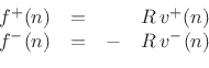 , equals the
net force acting to the right.
, equals the
net force acting to the right.
.
.
.
.
.
.
.
.
.
.
.
.
.
.
.
.
.
.
.
.
.
.
.
.
.
.
.
.
.
.
- ... junction.C.5
- When the wave impedance
is complex, the junction effectively has state, so that energy, but not
necessarily power, is conserved. See §C.18 for an example.
.
.
.
.
.
.
.
.
.
.
.
.
.
.
.
.
.
.
.
.
.
.
.
.
.
.
.
.
.
.
- ... coefficient.C.6
- We
previously have denoted reflection coefficients by
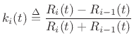 and
and  ,
where `r' stands for ``reflection.'' We now start using
,
where `r' stands for ``reflection.'' We now start using  because
it is most commonly used in the literature for ladder and lattice
digital filters [299]. Be careful, however, because
is also
the standard notation for wave number (spatial radian
frequency) in the field of acoustics, i.e.,
because
it is most commonly used in the literature for ladder and lattice
digital filters [299]. Be careful, however, because
is also
the standard notation for wave number (spatial radian
frequency) in the field of acoustics, i.e.,
 where
denotes wavelength (spatial period in meters).
Normally
will not be subscripted when it denotes wavenumber, but we
saw even that in §C.8.1 above.
where
denotes wavelength (spatial period in meters).
Normally
will not be subscripted when it denotes wavenumber, but we
saw even that in §C.8.1 above.
.
.
.
.
.
.
.
.
.
.
.
.
.
.
.
.
.
.
.
.
.
.
.
.
.
.
.
.
.
.
- ...
scattering.C.7
- Here it is assumed that
 and
and  in
the Kelly-Lochbaum junction can be computed exactly from
in the
number system being used. This is the case in two's complement
arithmetic as is typically used in practice.
in
the Kelly-Lochbaum junction can be computed exactly from
in the
number system being used. This is the case in two's complement
arithmetic as is typically used in practice.
.
.
.
.
.
.
.
.
.
.
.
.
.
.
.
.
.
.
.
.
.
.
.
.
.
.
.
.
.
.
- ... waveguides.C.8
- This
section is adapted from [438,437].
.
.
.
.
.
.
.
.
.
.
.
.
.
.
.
.
.
.
.
.
.
.
.
.
.
.
.
.
.
.
- ...
``right-going.''C.9
- In the acoustic tube literature which
involves only a cascade chain of acoustic waveguides,
 is
taken to be traveling to the right along the axis of the tube
[299]. In classical network theory [35] and in
circuit theory, velocity (current) at the terminals of an
-port
device is by convention taken to be positive when it flows into
the device.
is
taken to be traveling to the right along the axis of the tube
[299]. In classical network theory [35] and in
circuit theory, velocity (current) at the terminals of an
-port
device is by convention taken to be positive when it flows into
the device.
.
.
.
.
.
.
.
.
.
.
.
.
.
.
.
.
.
.
.
.
.
.
.
.
.
.
.
.
.
.
- ...
NotesC.10
- This section was added August 2023 for the next (third) printing
of the 2010 edition, since it contains nothing new since 2010, in principle.
.
.
.
.
.
.
.
.
.
.
.
.
.
.
.
.
.
.
.
.
.
.
.
.
.
.
.
.
.
.
- ...
NotesC.11
- This section was added August 2023 for the next (third) printing
of the 2010 edition, since it contains nothing new since 2010, in principle.
.
.
.
.
.
.
.
.
.
.
.
.
.
.
.
.
.
.
.
.
.
.
.
.
.
.
.
.
.
.
- ...BankAndMattiDAFX10:C.12
- The
instantaneous and delayed biquad components are readily derived
from looking at
![$ B(z)/A(z) = b_0 + [B(z)-b_0A(z)]/A(z)$](img3989.png) . More general
cases can be computed in matlab using the residued function [452]:
https://ccrma.stanford.edu/~jos/filters/FIR_Part_PFE.html.
. More general
cases can be computed in matlab using the residued function [452]:
https://ccrma.stanford.edu/~jos/filters/FIR_Part_PFE.html.
.
.
.
.
.
.
.
.
.
.
.
.
.
.
.
.
.
.
.
.
.
.
.
.
.
.
.
.
.
.
- ... foundC.13
- http://ccrma.stanford.edu/~jos/filters/Similarity_Transformations.html
.
.
.
.
.
.
.
.
.
.
.
.
.
.
.
.
.
.
.
.
.
.
.
.
.
.
.
.
.
.
- ... magnitude:C.14
- While the
literature seems to mention this property only for prime numbers
,
it is straightforward to show that it holds in fact for all positive odd
integers
. Prime values of
have advantages, however, when harmonics
of the ``design frequency'' are considered.
.
.
.
.
.
.
.
.
.
.
.
.
.
.
.
.
.
.
.
.
.
.
.
.
.
.
.
.
.
.
- ...CoxEtAl06.C.15
- Footnote added 2018-01-28:
New ultra-thin quadratic residue diffusers, using acoustic resonance
in place of propagation delay to achieve desired phase shifts, thereby
reducing the depth of the diffuser array by 90%, are described at
https://journals.aps.org/prx/pdf/10.1103/PhysRevX.7.021034.
.
.
.
.
.
.
.
.
.
.
.
.
.
.
.
.
.
.
.
.
.
.
.
.
.
.
.
.
.
.
- ...
algorithms.C.16
- See [105] for discussion of a wider
variety of digital sine generation methods.
.
.
.
.
.
.
.
.
.
.
.
.
.
.
.
.
.
.
.
.
.
.
.
.
.
.
.
.
.
.
- ... algorithm,C.17
- The
``magic circle'' algorithm is so named because it generates closed
curves in the
 plane even when numerical precision is
very low. For this reason, it has long been used as an algorithm
for drawing ``circles'' (actually ellipses) in computer graphics.
The algorithm is derived naturally by numerically integrating the
derivative relationships between sine and cosine:
plane even when numerical precision is
very low. For this reason, it has long been used as an algorithm
for drawing ``circles'' (actually ellipses) in computer graphics.
The algorithm is derived naturally by numerically integrating the
derivative relationships between sine and cosine:
The magic circle algorithm is easily shown to be equivalent to the
lowpass output of the infinite- second-order digital state variable
filter in ``Chamberlin form'' (defined
in, e.g., [480,79]).
second-order digital state variable
filter in ``Chamberlin form'' (defined
in, e.g., [480,79]).
.
.
.
.
.
.
.
.
.
.
.
.
.
.
.
.
.
.
.
.
.
.
.
.
.
.
.
.
.
.
- ...
amplitude),C.18
- When
 is constant, the time constant
 of the ensuing exponential growth or decay may be found by
solving
of the ensuing exponential growth or decay may be found by
solving
 for
to obtain
for
to obtain
 ln
ln , where
denotes the sampling interval, and
ln
denotes the natural
logarithm of
.
, where
denotes the sampling interval, and
ln
denotes the natural
logarithm of
.
.
.
.
.
.
.
.
.
.
.
.
.
.
.
.
.
.
.
.
.
.
.
.
.
.
.
.
.
.
.
- ... analysisC.19
- http://ccrma.stanford.edu/~jos/filters/State_Space_Models.html
.
.
.
.
.
.
.
.
.
.
.
.
.
.
.
.
.
.
.
.
.
.
.
.
.
.
.
.
.
.
- ... velocity.C.20
- More precisely,
it could be expressed as
![$ [{\dot u}(t,x)+{\ddot u}(t,x)\,dx]/2$](img4347.png) , but this introduces
a term that is second-order in
, but this introduces
a term that is second-order in 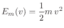 that would ultimately be
dropped.
that would ultimately be
dropped.
.
.
.
.
.
.
.
.
.
.
.
.
.
.
.
.
.
.
.
.
.
.
.
.
.
.
.
.
.
.
- ... network.F.1
- Wave
digital filters are not the same thing as digital waveguide networks,
however, because the wave variables in a wave digital filter have a
compressed frequency spectrum (from the bilinear transform), while the
signals in a digital waveguide network have a bandlimited spectrum
which is not warped.
.
.
.
.
.
.
.
.
.
.
.
.
.
.
.
.
.
.
.
.
.
.
.
.
.
.
.
.
.
.
- ...
waveguideF.2
- Here, it is perhaps most concrete to think in terms
of electrical equivalent circuits, so that the mass is an inductor and
a ``waveguide'' is a ``transmission line.''
.
.
.
.
.
.
.
.
.
.
.
.
.
.
.
.
.
.
.
.
.
.
.
.
.
.
.
.
.
.
- ... mass,F.3
- The phase delay,
for example, of the reflectance
 of an ideal spring is
given by
of an ideal spring is
given by
At  rad/sec, in particular,
the phase delay is
rad/sec, in particular,
the phase delay is
![$ P(1)=-\angle[(1-j)/(1+j)]=-\angle(-j) = \pi/2$](img5043.png) .
Since the period is
when
, this is a quarter-cycle
of delay.
.
Since the period is
when
, this is a quarter-cycle
of delay.
After the bilinear transform
 , the phase delay becomes
where  is defined by
 (the
relationship between continuous-time frequency and discrete-time
frequency imposed by the bilinear transform). Thus, the phase delay
comes out to exactly one sample at each frequency. Checking the point
(the
relationship between continuous-time frequency and discrete-time
frequency imposed by the bilinear transform). Thus, the phase delay
comes out to exactly one sample at each frequency. Checking the point
 ,
i.e., four samples per period, we find that one sample of delay does
in fact correspond to a quarter-cycle of delay.
,
i.e., four samples per period, we find that one sample of delay does
in fact correspond to a quarter-cycle of delay.
The same holds true for the group delay of the spring reflectance:
We see that the frequency-warping under the bilinear transform serves
to move each frequency to the unique point along the unit circle at
which the reflectance of a mass or spring happens to be exactly one
sample. The mass reflectance additionally inverts.
.
.
.
.
.
.
.
.
.
.
.
.
.
.
.
.
.
.
.
.
.
.
.
.
.
.
.
.
.
.
- ...tankwdf.F.4
- Note that the wave
variables are now labeled in element-centric notation as opposed to
adaptor-centric notation:
.
.
.
.
.
.
.
.
.
.
.
.
.
.
.
.
.
.
.
.
.
.
.
.
.
.
.
.
.
.
- ... limit.F.5
- Note that the mass and
velocity limits are tied together such that
 constant. This
information is lost in the final limits because the expression
constant. This
information is lost in the final limits because the expression
 is ``indeterminate''.
.
.
.
.
.
.
.
.
.
.
.
.
.
.
.
.
.
.
.
.
.
.
.
.
.
.
.
.
.
.
- ...SmithLAC08.H.1
- http://ccrma.stanford.edu/realsimple/faust_strings
.
.
.
.
.
.
.
.
.
.
.
.
.
.
.
.
.
.
.
.
.
.
.
.
.
.
.
.
.
.


![$\displaystyle \frac{e^2}{(r+\Delta r)^2}
= \frac{e^2}{r^2}\left(1+\frac{\Delta r}{r}\right)^{-2}
= \frac{e^2}{r^2}\left[1-2\frac{\Delta r}{r} + {\cal O}\left(\frac{\Delta r}{r}\right)^2\right]
\approx \frac{e^2}{r^2} +
\underbrace{\left(-\frac{2}{r^3}\right)}_k\Delta r,
$](img2643.png)