We have thus far considered discrete-time simulation of transverse
displacement ![]() in the ideal string. It is equally valid to
choose velocity
in the ideal string. It is equally valid to
choose velocity
![]() , acceleration
, acceleration
![]() , slope
, slope ![]() , or perhaps some other derivative
or integral of displacement with respect to time or position.
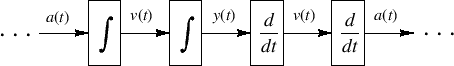
Conversion between various time derivatives can be carried out by
means integrators and differentiators, as depicted in
Fig.C.10. Since integration and
differentiation are linear operators, and since the traveling
wave arguments are in units of time, the conversion formulas relating
, or perhaps some other derivative
or integral of displacement with respect to time or position.
Conversion between various time derivatives can be carried out by
means integrators and differentiators, as depicted in
Fig.C.10. Since integration and
differentiation are linear operators, and since the traveling
wave arguments are in units of time, the conversion formulas relating
![]() ,
, ![]() , and
, and ![]() hold also for the traveling wave components
hold also for the traveling wave components
![]() .
.
![\includegraphics[scale=0.9]{eps/fwaveconversions}](img3446.png) |
Differentiation and integration have a simple form in the
frequency domain. Denoting the Laplace Transform of ![]() by
by
 |
(C.36) |
| (C.37) |
In discrete time, integration and differentiation can be accomplished using digital filters [365]. Commonly used first-order approximations are shown in Fig.C.12.
![\includegraphics[width=\twidth]{eps/fdigitaldiffint}](img3451.png) |
If discrete-time acceleration ![]() is defined as the sampled version of
continuous-time acceleration, i.e.,
is defined as the sampled version of
continuous-time acceleration, i.e.,
![]() , (for some fixed continuous position
, (for some fixed continuous position ![]() which we
suppress for simplicity of notation), then the
frequency-domain form is given by the
which we
suppress for simplicity of notation), then the
frequency-domain form is given by the ![]() transform
[488]:
transform
[488]:
 |
(C.38) |
In the frequency domain for discrete-time systems, the first-order approximate conversions appear as shown in Fig.C.13.
![\includegraphics[scale=0.6]{eps/ffddigitaldiffint}](img3455.png) |
The ![]() transform plays the role of the Laplace transform for discrete-time
systems. Setting
transform plays the role of the Laplace transform for discrete-time
systems. Setting ![]() , it can be seen as a sampled Laplace
transform (divided by
, it can be seen as a sampled Laplace
transform (divided by ![]() ), where the sampling is carried out by halting
the limit of the rectangle width at
), where the sampling is carried out by halting
the limit of the rectangle width at ![]() in the definition of a Reimann
integral for the Laplace transform. An important difference between the
two is that the frequency axis in the Laplace transform is the imaginary
axis (the ``
in the definition of a Reimann
integral for the Laplace transform. An important difference between the
two is that the frequency axis in the Laplace transform is the imaginary
axis (the ``![]() axis''), while the frequency axis in the
axis''), while the frequency axis in the ![]() plane is on
the unit circle
plane is on
the unit circle
![]() . As one would expect, the frequency axis for
discrete-time systems has unique information only between frequencies
. As one would expect, the frequency axis for
discrete-time systems has unique information only between frequencies
![]() and
and ![]() while the continuous-time frequency axis extends to plus and
minus infinity.
while the continuous-time frequency axis extends to plus and
minus infinity.
These first-order approximations are accurate (though scaled by ![]() )
at low frequencies relative to half the sampling rate, but they are
not ``best'' approximations in any sense other than being most like
the definitions of integration and differentiation in continuous time.
Much better approximations can be obtained by approaching the problem
from a digital filter design viewpoint, as discussed in §8.6.
)
at low frequencies relative to half the sampling rate, but they are
not ``best'' approximations in any sense other than being most like
the definitions of integration and differentiation in continuous time.
Much better approximations can be obtained by approaching the problem
from a digital filter design viewpoint, as discussed in §8.6.
![\includegraphics[scale=0.9]{eps/ffdwaveconversions}](img3450.png)