 |
Flanging is a delay effect that has been available in recording studios since at least the 1960s. Surprisingly little literature exists, although there is some [32,433,59,17,104,244].6.1
The ``flanging'' effect can be understood by considering two tape machines set up to play the same tape in unison, with their outputs added together (mixed equally), as shown in Fig.5.2. To create the flanging effect, the flange of one of the supply reels can touched lightly to make it play a littler slower. This causes a delay to develop between the two tape machines. The flange is released, and the flange of the other supply reel is touched lightly to slow it down. This causes the delay to gradually disappear and then begin to grow again in the opposite direction. The delay is kept below the threshold of echo perception (e.g., only a few milliseconds in each direction). The process is repeated as desired, pressing the flange of each supply reel in alternation. The flanging effect has been described as a kind of ``whoosh'' passing subtly through the sound.6.2The effect is also compared to the sound of a jet passing overhead, in which the direct signal and ground reflection arrive at a varying relative delay [59]. If flanging is done rapidly enough, an audible Doppler shift is introduced which approximates the ``Leslie'' effect commonly used for organs (see §5.9).
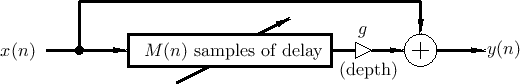
Flanging is modeled quite accurately as a feedforward comb filter, as
discussed in §2.6.1, in which the delay ![]() is varied
over time. Figure 5.3 depicts such a model. The input-output
relation for a basic flanger can be written as
is varied
over time. Figure 5.3 depicts such a model. The input-output
relation for a basic flanger can be written as
As shown in Fig.2.25, the frequency response of Eq.(5.1)
has a ``comb'' shaped structure. For ![]() , there are
, there are ![]() peaks in the frequency response, centered about frequencies
peaks in the frequency response, centered about frequencies
For
As is evident from Fig.2.25, at any given time there are ![]() notches in the flanger's amplitude response (counting positive-
and negative-frequency notches separately). The notches are thus
spaced at intervals of
notches in the flanger's amplitude response (counting positive-
and negative-frequency notches separately). The notches are thus
spaced at intervals of ![]() Hz, where
Hz, where ![]() denotes the sampling
rate. In particular, the notch spacing is inversely
proportional to delay-line length.
denotes the sampling
rate. In particular, the notch spacing is inversely
proportional to delay-line length.
The time variation of the delay-line length ![]() results in a
``sweeping'' of uniformly-spaced notches in the spectrum. The
flanging effect is thus created by moving notches in the
spectrum. Notch motion is essential for the flanging effect. Static
notches provide some coloration to the sound, but an isolated notch
may be inaudible [140]. Since the steady-state sound
field inside an undamped acoustic tube has a similar set of
uniformly spaced notches (except at the ends), a static row of notches
tends to sound like being inside an acoustic tube.
results in a
``sweeping'' of uniformly-spaced notches in the spectrum. The
flanging effect is thus created by moving notches in the
spectrum. Notch motion is essential for the flanging effect. Static
notches provide some coloration to the sound, but an isolated notch
may be inaudible [140]. Since the steady-state sound
field inside an undamped acoustic tube has a similar set of
uniformly spaced notches (except at the ends), a static row of notches
tends to sound like being inside an acoustic tube.
