Answers

• To what types of systems can wave digital and digital waveguide network simulation approaches be applied?

Let us first confine our attention to numerical methods which result from the passive discretization of an MDKC; all the methods discussed in this thesis are of this form, except for the multigrid methods of §4.9, the type I and II DWNs for the transmission-line and parallel-plate problems (see §4.3.6 and §4.4.2, respectively), the DWN for the Euler-Bernoulli beam system (see §5.1) and the Timoshenko beam systems of §5.2.3. We can then rephrase our question as: For which types of systems do there exist passive MDKC representations?

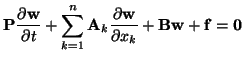
In general, MDKC representations follow directly only for $(n+1)$D symmetric hyperbolic systems of the form of (3.1), and we repeat this definition here.

$${\bf P}\frac{\partial {\bf w}}{\partial t} +\sum_{k=1}^{n}{\bf A}_{k}\frac{\partial {\bf w}}{\partial x_{k}} + {\bf Bw} + {\bf f} = {\bf0}$$ (6.1)

Recall that the coupling matrices ${\bf A}_{k}$ are constrained to be symmetric and constant, so all material parameter variation is confined to the symmetric positive-definite matrix coefficient ${\bf P}$ of the time derivatives, and the coefficient ${\bf B}$ of the constant-proportional terms. (Indeed, ${\bf B}$ can be time-varying without affecting the network representation of any system in which it appears. We will look at the more useful case of time variation of ${\bf P}$, which occurs in, e.g., time-varying vocal tract models [145], in §6.2.7.) For passivity, we generally require that the symmetric part of ${\bf B}$ be positive semi-definite. The symmetry of the ${\bf A}_{k}$ implies a network representation involving only reciprocal reactive MD circuit elements. In fact, the structure of the ${\bf A}_{k}$ directly specifies the MD network topology; if any of the ${\bf A}_{k}$ contains a non-zero entry in the $(p,q)$th position, then we will necessarily have some coupling between the $p$th and $q$th loops in the network representation. The constancy of the ${\bf A}_{k}$ has important implications for the energetic analysis of the system, as we saw in §3.2, and also ensures that all inter-loop couplings can be accomplished through the use of linear and shift-invariant (LSI) coupling elements (generally the Jaumann or lattice two-ports introduced in §3.7.2 for MDWDFs, or the alternative hybrid form of §4.10 for DWNs). This is crucial, because the spatial derivative information is concentrated in these coupling elements; discretization of a reactive element is usually only passive if its defining parameters (usually inductances) are independent of the integration directions. (The main exceptions here are the reactive elements discussed at the end of §3.5.1; such elements can be used in the time-varying case, as mentioned above, or in nonlinear problems, which we will discuss at length in Appendix B.) In fact, all the MD-passive systems we have examined have networks which can be decomposed into two networks as in Figure 6.1. The subnetwork on the left is made up of a set of time inductors (or capacitors) with spatially-varying inductances (or capacitances), and perhaps resistances and can be discretized through the trapezoid rule in time. In the expanded signal-flow graphs, these always give rise to self-loops. The right-hand subnetwork is linear and shift-invariant, and contains all the spatial derivative terms, in the form of Jaumann or lattice connections, for MDWDFs, or the hybrid form for DWNs, discussed in §4.10. It can be discretized by the MD trapezoid rule (or alternative spectral mappings, for DWNs), and the full discrete network will be passive if the subnetworks are MD-passive separately.

Figure 6.1: Network decomposition of passive symmetric hyperbolic systems.

A few other features are worthy of comment. First, although the ${\bf P}$ matrix is diagonal for many of the systems we have looked at, it is not for any of the vibrating elastic systems in (2+1)D and (3+1)D of Chapter 5 (nor will it be for, say, Maxwell's equations in anisotropic media, or mutually inductive coupled transmission lines, or systems in general curvilinear coordinate systems). The non-diagonal elements of ${\bf P}$ are modeled in an MDKC as mutual inductances or capacitances, and subsequently require vector scattering junctions, as discussed in §2.3.7. This leads to more complex ``block'' scattering matrices, but passivity is not compromised. Second, consider the ${\bf B}$ matrix, which is not constrained to be of any particular form. If the symmetric part of ${\bf B}$ is positive semi-definite, then it always implies loss, and can be realized as a purely resistive coupling network. The anti-symmetric part of ${\bf B}$, which does not produce loss, gives rise to dispersion (as for the Timoshenko beam in §5.2, the Mindlin plate in §5.4 and the shell models of §5.5), and corresponds to lossless gyrator couplings among the circuit loops. In general, if the ${\bf B}$ matrix is not sparse, the resulting resistive and gyrator couplings in the MDKC may considerably complicate the resulting discrete network (i.e., various reflection-free ports will be required). Third, the system (6.1) forms a subclass of what are called strongly hyperbolic systems, for which the initial value problem is well-posed [82]. A general strongly hyperbolic also can be written in the form of (6.1), but the matrices ${\bf A}_{k}$ are not constrained to be symmetric (any real linear combination of the ${\bf A}_{k}$ must, however, possess a set of real distinct eigenvalues). If the ${\bf A}_{k}$ can not be simultaneously symmetrized by some change of variables, then it is clear that the set of reactive reciprocal circuit elements does not suffice for a passive circuit representation, even though energy estimates of the type discussed in §3.2 may be available. It would be quite interesting to know how a network could be designed for such strongly, but not symmetric hyperbolic systems. Furthermore, system (6.1) is not even the most general form of symmetric hyperbolic system. The matrices ${\bf A}_{k}$ may be functions of space or time variables, though the simple energetic analysis of §3.2 becomes more involved; passivity does not immediately follow. Fourth, we included a discussion of a DWN for the Euler-Bernoulli system in §5.1, in order to indicate that such networks may be available even if the physical system is not hyperbolic (group velocities are unbounded for the classical beam model). Such extensions of scattering methods have also been discussed in the MDWD context in [202]. Fifth, for nonlinear systems, the natural extension of symmetric hyperbolicity which leads to circuit representations is skew self-adjointness. We will examine such extensions in Appendix B.

• What features do the two methods share, and what distinguishes them?

The most basic difference between the two methods is, as we emphasized early on in Chapter 1, that a DWN can always be viewed as a large network of scattering junctions, connected to one another port-wise by bidirectional delay lines; a MDWD network is better thought of as the discrete image of a multidimensional Kirchoff circuit representation (MDKC). Though a signal flow graph for a MDWD network follows immediately, it can not be decomposed into a collection of discrete transmission lines, or bidirectional delay lines. Both methods, however, operate using exclusively scattering and shifting operations--it may be useful to flip to Figure 4.44, which shows the expanded signal flow graphs for the DWN and MDWD networks for the (1+1)D transmission line equations. Notice that the port-wise connectivity of the MDWD network is always lost in this (and all) expanded forms; for certain adaptors, the two wave signal paths entering the ``port'' are not connected to the two terminals of another single port. We have seen, of course, in §4.10, that many DWN forms operating on regular grids can also be derived from MD circuit representations; DWNs are more general in the sense they may be constructed completely locally, and in irregular arrangements (recall the general discussion of DWNs in §1.1.2), without using an MDKC.

We have also seen, in the first few sections of Chapter 4, that DWNs are in general equivalent to simple two-step centered finite difference schemes of the FDTD variety. In §3.9, we showed that MDWD simulation methods also correspond to finite difference schemes, but they are in general multi-step methods. In both cases, the calculations have been rearranged (using wave variables) in a one-step form. If the underlying system is lossless, and power-normalized wave variables are employed, then at any time step the discrete network recursion involves an orthogonal transformation (scattering) applied to the entire set of wave variables stored in memory, followed by a permutation (shifting) operation. Losslessness, and thus stability is thus ensured in a very direct way. The two methods possess distinct spectral properties, which we examined briefly in the case of the (1+1)D transmission line in §4.3.8.

There is another more subtle distinction. For almost all first-order PDE systems that follow from physical laws, the state variables can be separated into two types which are dual to one another. To be more precise, in all the systems of the form of (6.1) which we have examined in this thesis, the time derivative of a variable of one type is always related to spatial derivatives of variables of the other type; for example, voltages and currents are dual variables in the transmission line and parallel-plate problems, as are electric and magnetic field components described by Maxwell's equations (4.110), etc. This duality implies a certain structure in the coupling matrices ${\bf A}_{k}$. In the MDKCs developed by Fettweis et al., however, this structure is ignored, and all variables are treated generally as currents. In the resulting numerical methods, this usually implies that all the dependent variables are computed together at the same spatial locations, and at all time steps. (As we mentioned in §3.9, however, it is possible to design MDWD simulation methods operate on ``checkerboard'' grids; the variables are all computed together, but at locations interleaved in time and space.) For the DWNs we discussed in Chapters 4 and 5, we have made use of this duality in order to design networks in which the two sets of variables are computed at alternating time instants and spatial locations. One set is interpreted as current-like, and the other as voltage-like. The resulting alternations are generally indicated by grey/white junction colorings in the signal flow graphs. (It is worth calling attention, at this point, to the analogous distinction between so-called ``expanded'' and ``condensed'' node TLM formulations [29].)

• What are their relative advantages?

The answers to the previous question have several practical implications.

Because any DWN always can be written in the form of a large network of port-wise connected scattering junctions, passive (and thus stable) boundary termination is straightforward. For the transmission line (see §4.3.9), the parallel-plate problem (see §4.4.4), beams (see §5.1.3 and §5.2.4) and plates (see §5.4.2), many useful lossless boundary conditions can be effected through the use of simple short- or open-circuit, or self-loops connected to scattering junctions which lie on the boundary. In fact, the termination of any boundary junction with an all-pass (more generally bounded real) scattering one-port will always yield a numerical scheme which is guaranteed lossless (more generally passive), though the physical interpretation of such an arbitrary termination may not be obvious. It is worth emphasizing that the ease with which passivity (or exact losslessness, if so desired) can be ensured in the presence of boundary conditions is one great benefit of a scattering formulation. It can be quite difficult to ensure the stability of a boundary condition applied to a finite difference scheme. The same is not true of MDWD networks; because port-wise connectivity is lost in the expanded signal-flow graph, passive termination is no longer simple or straightforward. We indicated in §3.11 and §5.2.4 the severe difficulties inherent in the ``wave-canceling'' termination approach described in the literature [107], and will look at a possible theoretical foundation for passive distributed network termination shortly in §6.2.3.

An MDKC is always mapped, via spectral transformations or integration rules, to a discrete time and space MDWD image network. As we mentioned above, the resulting numerical method always operates on a regular grid in some coordinate system. It is thus impossible, through the approach of Fettweis et al., to arrive at structures which operate on irregular grids. As we have seen in §4.9, because DWNs may be constructed locally, multigrid methods become a possibility--DWNs of differing densities or in different coordinate systems may be simply connected to one another, in such a way that passivity is maintained across the interface. Such interfaces can be designed so as to be locally consistent with the underlying model problem; as a result, numerical reflection vanishes as the grid spacings become small. The applications to numerical integration over irregular problem domains should be self-evident.

• Can they be unified in a formal way?

The single most satisfying result in this thesis was the successful ``merging'' of waveguide networks and MDWDFs in §4.10. A passive MDKC representation of a system of PDEs is no more than that--a representation. It illustrates, however, how the system can be decomposed into simpler elements, each of which is passive in its own right, and immediately suggests a stable numerical scheme. Each element can be discretized through the application of one or a set of spectral mappings, or multidimensional integration rules, in such a way that this passivity is preserved (this is discussed in §3.5.3) in a discrete network, which can then be directly implemented as a computer simulation routine. The MD trapezoid rule, or bilinear transform, which gives rise to wave digital networks, is one such rule but is by no means the only way of proceeding; in multiple dimensions, the family of such mappings is large and diverse. Digital waveguide networks are the result of the application of another member of this family. As we have seen, especially in Chapter 5, digital waveguide networks are now applicable to any system that has been approached using MDWDFs (we have covered most of them in this thesis). We will make some more comments on this subject in the §6.2.5, but at this stage, the author feels justified in lumping these techniques together as simply ``wave'' or ``scattering'' methods.

Figure 6.2: The generalized family of passive numerical methods.

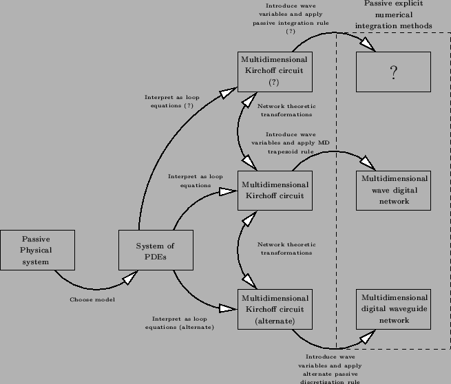
As indicated in Figure 6.2, the unification of these two methods also implies their membership within a larger class of passive numerical methods; indeed, any set of passive spectral mappings or integration rules may be applied to any circuit representation of a system of PDEs, and the result is necessarily a stable numerical method built of the same basic scattering and shifting operations as the DWN or an MDWD network. We refer to §6.2.5 for a few further comments on this subject.

• What extensions and improvements can be made to the existing forms of these methods?

For all stable explicit numerical methods for hyperbolic systems, a CFL-type condition must necessarily be obeyed. That is, if the time step is $T$, and the grid spacing is $\Delta$, then we will require

$$T\leq \kappa\gamma_{max}\Delta$$ (6.2)

where $\gamma_{max}$ is the maximum local group velocity of the system, as defined in §3.2. In other words, the physical region of dependence of the problem must be contained within the region of dependence of the recursion. The parameter $\kappa$ is some constant which depends on problem specifics, such as the number of spatial dimensions, the width of the computational stencil of the scheme, etc., but not the material parameter values themselves. One serious shortcoming of the MDWD numerical methods proposed by Fettweis et al. is that for a given grid spacing, the maximum time-step allowed may be a good deal smaller than the optimal CFL bound, if there are spatial variations in the physical medium. As we have seen in §5.2.1, this constraint on the time step becomes especially severe for stiff vibrating systems. We showed in §3.12 and §5.2.6 how balancing approaches may be used to derive networks which give rise to numerical methods which are optimal in that a bound of the type (6.2) is satisfied. Certain DWNs (in particular, the type I and II forms for the transmission line, parallel-plate systems) also exhibit this optimality property, though such forms do not follow directly from MDKC representations that we have discussed.

The DWN has been applied, in the past, to problems in musical acoustics and physical modeling. In particular, DWNs have been used to solve the wave equation in one, (uniform strings and acoustic tubes) two (membranes), or three (room acoustic) spatial dimensions. We have looked at numerous ways of extending the DWN to deal with more realistic problems. First, from the result in §4.10, the DWN is now applicable to a wide class of physical systems, and in particular, those which may exhibit material parameter variation. Among them are the transmission line and parallel-plate problems (which are analogous to strings and membranes, of varying density), and the many elastic solid systems discussed in Chapter 5. In fact, DWNs are fully as general as the MDWD simulation networks of Fettweis, and possess all the same good numerical properties; because boundary conditions are easier to deal with, one might go so far as to say that they are a superior form of scattering method. Second, we examined ways of dealing with boundary and initial conditions in a systematic way (as we mentioned above, this has not been done for MDWD networks). Third, we introduced DWN formulations appropriate for problems with irregular boundary configurations; waveguide meshes in transformed coordinates and multigrid forms are two possibilities. Fourth, we examined the possibilities of higher-order spatially accurate DWNs which follow directly from an MDKC representation. Fifth, we will spend some time in Appendix A cataloging the many forms of waveguide mesh which have been proposed, and looking into ways of improving their numerical dispersion behavior.