Next: Type I: Voltage-centered Mesh
Up: The Waveguide Mesh
Previous: The Waveguide Mesh
Losses, Sources, and Spatially-varying Coefficients
We can deal with spatially-varying material parameters as well as losses and sources in a manner similar to the (1+1)D case. The full (2+1)D transmission line equations, as originally presented in §3.8, are
 |
(4.70a) |
where we have
 and
and
 , and
, and  ,
,  and
and  are driving functions of
  ,
,  and
and  .
.
The centered difference approximation to (4.58) is
where
for  ,
,  half-integer such that
  is odd, and
for  ,
,  integer. For the sources, we have used
where
Again, we have applied a semi-implicit approximation to the constant-proportional terms of (4.58).
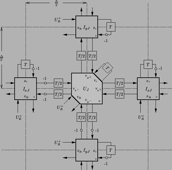
The waveguide network shown in Figure 4.21 is a direct generalization to (2+1)D of Figure 4.15. To the structure of Figure 4.20 we have added an extra port to each scattering junction, series or parallel, which is connected to a self-loop of impedance  and doubled delay length, as well as a port with impedance
  to introduce losses and sources. All immittances are indexed by the coordinates of their associated junctions. As before, we set the admittance
  =
=  for any impedance
  in the network. In Figure 4.21, the linking admittances of the bidirectional delay lines are indicated only at the parallel junction, since we must have
The junction admittances and impedances are thus
Beginning from series and parallel junctions, and proceeding through derivations similar to (4.32) yields the difference scheme (4.59) in the junction variables  ,
,  and
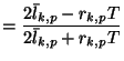
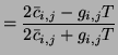
and  , provided we set
Figure:
(2+1)D waveguide mesh for the varying-coefficient system (4.58), with losses and sources.
 |
We can again identify three useful ways of setting the immittances:
Next: Type I: Voltage-centered Mesh
Up: The Waveguide Mesh
Previous: The Waveguide Mesh
Stefan Bilbao
2002-01-22