Varying Coefficients

We now return to the more general case in which the material parameters $l$ and $c$ have spatial dependence. The staggered, or interleaved network of delay lines and scattering junctions presented in the last section gives rise to a centered difference method which approximates the solution to system (4.17). Consider the waveguide network in Figure 4.14.

Figure 4.14: Waveguide network for the (1+1)D transmission line equations with spatially-varying coefficients.

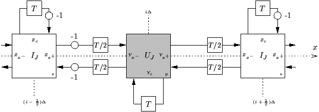
The picture is the same as in the constant-coefficient case, except that we have added an extra port to each scattering junction, which is connected to a delay line of impedance $Z_{c}$ (marked as $Y_{c}$ at the parallel junctions). These self-loops [167] are bidirectional delay lines in their own right--since both ends are connected to the same junction, we are free to drop one of the line pairs. Note that the loop connected to the series junction contains a sign inversion (like a lumped wave digital inductor) and the loop at the parallel junction does not (like a capacitor). Also note that the delay in this line is a full sample, so that we are able to operate on the interleaved grid. The reason for this choice should be clear from Figure 4.7. Now, the immittances of the delay lines are in general no longer identical, so we expect non-trivial scattering to occur, due to the spatially-varying material parameters. The admittances of the lines connected to the parallel junction at grid point $i$, $i$ integer, are denoted by $Y_{x^{+},i}$, $Y_{x^{-},i}$ and $Y_{c,i}$. The impedances of the self-loops at grid points $i+\frac{1}{2}$ for $i$ integer will be called $Z_{c,i+\frac{1}{2}}$. (We have marked these new immittances in Figure 4.14.) The junction immittances are now

$$Y_{J,i} \triangleq Y_{x^{+},i}+Y_{x^{-},i}+Y_{c,i}\hspace{0.5in}$$ Parallel junction

$$Z_{J,i+\frac{1}{2}} \triangleq Z_{x^{+},i+\frac{1}{2}}+Z_{x^{-},i+\frac{1}{2}}+Z_{c,i+\frac{1}{2}}\hspace{0.5in}$$ Series junction

$$= \frac{1}{Y_{x^{-},i+1}}+\frac{1}{Y_{x^{+},i}}+Z_{c,i+\frac{1}{2}}\notag$$

at parallel junctions at grid point $i$ and series junctions at grid point $i+\frac{1}{2}$, for integer $i$. We will call the new voltage wave variables entering and leaving the parallel junction from the new port $U_{c,i}^{+}(n)$ and $U_{c,i}^{-}(n)$ respectively, and those entering and leaving the series junction from its new port $U_{c,i+\frac{1}{2}}^{+}(n+{\textstyle \frac{1}{2}})$ and $U_{c,i+\frac{1}{2}}^{-}(n+{\textstyle \frac{1}{2}})$, for integer values of $i$ and $n$. In addition, we will adopt the notation

$$l_{k} \triangleq l(k\Delta)\hspace{1.0in}c_{k} \triangleq c(k\Delta)$$

for half-integer values of $k$.

One physical interpretation of the need for these self-loops is that if $l$ and $c$ vary over the domain, the effective local wave speed does as well. Thus, if we choose a regular grid spacing, there are necessarily grid points at which the space step/time step ratio is not the magic ratio (it must be greater, by the CFL criterion). Thus if we were to try to use a structure such as that pictured in Figure 4.12, regardless of how the waveguide impedances are set, energy would be moving ``too fast'' through the network. The extra delays at the junctions serve to slow down the propagation of energy, by storing a portion of it for a time step. The amount of slowdown is locally determined by the values of self-loop admittances and impedances. Self-loops are used for the same purpose in TLM [29,90]--in this context they are called inductive or capacitive stubs, depending on whether or not they invert sign.

Beginning from a parallel junction in Figure 4.14, we can proceed through a derivation similar to that leading to (4.31):

$$U_{J,i}(n) = \frac{2}{Y_{J,i}}\left( Y_{x^{+},i}U_{x^{+},i}^{+}(n)+Y_{x^{-},i}U_{x^{-},i}^{+}(n)+Y_{c,i}U_{c,i}^{+}(n)\right)\notag$$ (4.36)

$$= \frac{2}{Y_{J,i}}\left( I_{x^{+},i}^{+}(n)+I_{x^{-},i}^{+}(n)+Y_{c,i}U_{c,i}^{+}(n)\right)\notag$$ (4.37)

$$= \frac{2}{Y_{J,i}}\left( -I_{x^{-},i+\frac{1}{2}}^{-}(n-{\textstyl... ...^{+},i-\frac{1}{2}}^{-}(n-{\textstyle \frac{1}{2}})+I_{c,i}^{+}(n)\right)\notag$$ (4.38)

$$= \frac{2}{Y_{J,i}}\left( -I_{J,i+\frac{1}{2}}(n-{\textstyle \frac{1}{2}})+I_{J,i-\frac{1}{2}}(n-{\textstyle \frac{1}{2}})\right)\notag$$ (4.39)

$$\hspace{0.5in}+\hspace{0.1in} \frac{2}{Y_{J,i}}\left(I_{x^{-},i+\... ...+},i-\frac{1}{2}}^{+}(n-{\textstyle \frac{1}{2}})-I_{c,i}^{-}(n-1)\right)\notag$$ (4.40)

$$= \frac{2}{Y_{J,i}}\left( -I_{J,i+\frac{1}{2}}(n-{\textstyle \frac{1}{2}})+I_{J,i-\frac{1}{2}}(n-{\textstyle \frac{1}{2}})\right)\notag$$ (4.41)

$$\hspace{0.5in}-\hspace{0.1in} \frac{2}{Y_{J,i}}\left(I_{x^{+},i}^{-}(n-1)+I_{x^{-},i}^{-}(n-1)+I_{c,i}^{-}(n-1)\right)\notag$$ (4.42)

$$= \frac{2}{Y_{J,i}}\left( -I_{J,i+\frac{1}{2}}(n-{\textstyle \frac{1}{2}})+I_{J,i-\frac{1}{2}}(n-{\textstyle \frac{1}{2}})\right)+U_{J,i}(n-1)$$ (4.43)

In order to equate this difference relation with (4.22b), we must have, recalling (4.21b),

$$Y_{J,i} = 2v_{0}\bar{c}_{i}$$ (4.44)

Beginning from the series junctions at $x=(i+\frac{1}{2})\Delta$, for $i$ integer, we obtain similarly an interleaved central difference approximation to (4.17a), under the constraint

$$Z_{J,i+\frac{1}{2}} = 2v_{0}\bar{l}_{i+\frac{1}{2}}$$ (4.45)

Under the further condition that all impedances in the network be positive, these constraints give rise to a family of stable centered difference approximations to (4.17). We can distinguish three special types: