Centered Difference Schemes and Grid Decimation

Suppose we are interested in developing a finite difference scheme to calculate the solution to (4.17) numerically. We first define grid functions $I_{i}(n)$, and $U_{i}(n)$ which, for convenience, will run over half-integer values of $i$ and $n$, i.e.,

$$i,n = \hdots -1,-{\textstyle \frac{1}{2}},0,{\textstyle \frac{1}{2}},1\hdots$$

They are intended to approximate $i$ and $u$ at the points $(i\Delta,nT)$, where $\Delta$ is the spatial grid step, and $T$ the time step. We note that we have used the same variable, $i$, to stand for both the continuous-time current which solves (4.17), as well as the discrete-valued variable representing the spatial coordinate on the grid.

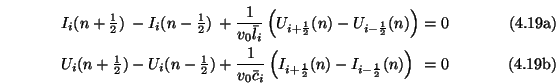
We have the centered difference approximations

$$\begin{eqnarray}\left.\frac{\partial w}{\partial t}\right\vert _{... ...2})\Delta,nT)-w((i-\frac{1}{2})\Delta,nT)}{\Delta}+O(\Delta^{2}) \end{eqnarray}$$ (4.19a)

where $w$ stands for either of $i$ or $u$.

Employing these differences in (4.17), and replacing the continuous time/space variables $i$ and $u$ by their respective grid functions yields the difference scheme

Here, we have chosen

for half-integer $i$. Because the centered difference approximations (4.19) are second-order accurate, $l$ and $c$ may be approximated to the same order without any decrease in accuracy. We leave the exact form of these approximations, $\bar{l}$ and $\bar{c}$ unspecified for the moment, but will return to various settings in §4.3.6. Also, in order to remain consistent with the notation in the MDWD schemes of the last chapter, we have set

$$v_{0} \triangleq \frac{\Delta}{T}$$

Thus difference equations (4.20) are consistent with (4.17), and accurate to $O(\Delta^{2},T^{2})$.

In a difference scheme for a general system of PDEs, it would be necessary to update all the grid functions every time step, and at every grid point--that is to say, at every increment in $n$ and $i$ of one-half, new values of the grid functions would have to be calculated, and indeed, we can proceed in this manner in with the scheme (4.20) as well. In this case, however, it is easy to see that updating $U_{k}(m)$, for $2k$ and $2m$ even requires access only to $I_{k}(m)$ at the previous time step, and at neighboring grid locations (thus for $2m$ odd and $2k$ odd), as well as $U$ at the same location, two time steps previously ($2m$ and $2k$ again even) [131,184]. Similarly, updating $I_{k}(m)$ for $2m$ odd and $2k$ odd involves only values of $U$ for $2m$ even and $2k$ even, and $I$ for $2m$ odd and $2k$ odd. It is then obvious that only values of $U_{k}(m)$ for which $2m$ is even and $2k$ even (and values of $I_{k}(m)$ with $2m$ odd and $2k$ odd) need enter into our scheme. We can thus decimate the grid in the manner shown in Figure 4.7.

Figure 4.7: Interleaved sampling grid for the (1+1)D transmission line.

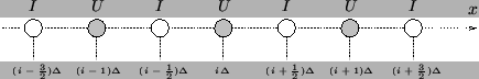We calculate the values of $U_{i}(n)$ at the grey dots in Figure 4.7, and $I_{i+\frac{1}{2}}(n+{\textstyle \frac{1}{2}})$ at the white dots. The difference scheme on the decimated grid can be written as

$$\begin{eqnarray}I_{i+\frac{1}{2}}(n+{\textstyle \frac{1}{2}}) - I... ...{2}})-I_{i-\frac{1}{2}}(n-{\textstyle \frac{1}{2}})\right) &=& 0 \end{eqnarray}$$ (4.22a)

for $i$, $n$ integer. We perform the calculation on the decimated grid with no decrease in accuracy, although we are of course approximating the solution at fewer grid points. In analogy with the continuous case, when $l$ and $c$ are constant it is possible to combine the difference equations (4.22) into a single equation for the voltage grid function $U$, which is

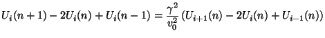$$U_{i}(n+1) -2U_{i}(n)+U_{i}(n-1) = \frac{\gamma^{2}}{v_{0}^{2}}\left(U_{i+1}(n)-2U_{i}(n)+U_{i-1}(n)\right)$$ (4.23)

and which solves the (1+1)D wave equation (4.18). For the so-called magic time step [184],

$$v_{0} = \gamma \triangleq \frac{1}{\sqrt{lc}}$$

the difference scheme (4.23) reduces to

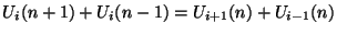$$U_{i}(n+1) + U_{i}(n-1) = U_{i+1}(n)+U_{i-1}(n)$$ (4.24)

a form which has great relevance to the discussion to follow on the waveguide implementation. It is interesting that in this case, the grid may be further decimated; we need only calculate $U_{i}(n)$ for $i+n$ even (or odd), for $i$, $n$ integer. We will examine this point in further detail in higher dimensions in Appendix A.