First-order System and the Wave Equation

We recall that the set of PDEs which describes the evolution of the voltage and current distributions along a lossless, source-free transmission line in (1+1)D is:

$$\begin{eqnarray}l\frac{\partial i}{\partial t} +\frac{\partial u}... ...rac{\partial u}{\partial t} +\frac{\partial i}{\partial x} &=& 0 \end{eqnarray}$$ (4.17a)

where $i(x,t)$ and $u(x,t)$ are, respectively, the current in and voltage across the lines, and $l(x)$ and $c(x)$, both assumed strictly positive everywhere, are the inductance and capacitance per unit length. For the moment, we will leave aside the discussion of boundary conditions, and deal only with the Cauchy problem (i.e., we assume the spatial domain of the problem to be the entire $x$ axis). Note also that this system includes the vocal tract model (1.20) as a special case, under an appropriate set of variable and parameter replacements.

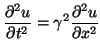
As discussed in §4.2.3, if we assume that $l$ and $c$ are constant, then the set of equations can be reduced to a single second order equation in the voltage alone:

$$\frac{\partial^{2} u}{\partial t^{2}} = \gamma^{2}\frac{\partial^{2} u}{\partial x^{2}}$$ (4.18)

where the wave speed $\gamma$ is given by

$$\gamma = \frac{1}{\sqrt{lc}}$$

This equation and its analogues in higher dimensions (see Appendix A) are collectively known as the wave equation. The solution, as mentioned in §4.2.3, can be written in terms of traveling waves. In the (1+1)D case, we can write an identical wave equation in the current alone, but this does not hold in higher dimensions.