Next: A General Approach: Multidimensional
Up: Digital Waveguide Networks
Previous: Waveguide Meshes and the
To answer this question, let us consider the two-dimensional waveguide mesh at a junction with coordinates  and
and  , for integer
  and
and  . The discrete-time junction pressure
 at time
  , for integer
  (recall that our digital waveguide network operates with a sampling period of
  ), can be written in terms of the four incident wave variables at the same location, from (1.14), as
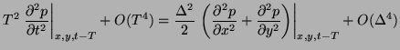
By tracing the propagation of the wave variables through the network backwards in time through two time steps, it is in fact possible to write a recursion in terms of the junction pressures alone,
 |
(1.17) |
Assume, for the moment, that these discrete time and space junction pressure signals are in fact samples of a continuous function  of
of  ,
,  and
and  . Expanding the terms in the recursion above in Taylor series about the location with coordinates and , at time
 gives
gives
Recalling that
 , where
  is the speed of wave propagation in the one-dimensional tubes, and discarding higher-order terms in and
  (they are assumed to be small), we get
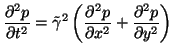 |
(1.18) |
This is simply the two-dimensional wave equation, with the wave speed
 defined by
 |
(1.19) |
This equation describes wave propagation in a lossless two-dimensional acoustic medium, and the DWN of Figure 1.8(b) can thus be considered to be a numerical integrator of this equation, assuming the wave speeds in the tubes are set according to (1.19); the discrete Huygens' principle interpretation of the behavior of the mesh is justified, at least in the limit as and become small . The recursion (1.17) in the junction pressures, however, can be seen as a simple finite difference scheme which could have been derived directly from (1.18) by replacing the partial derivatives by differences between values of a grid function
 on a numerical grid. Because the DWN operates using wave variables, we can see that the DWN is simply a different organization of the same calculation; in particular, it has been put into a form for which all operations (scattering, and shifting) rigidly enforce conservation of energy, in a discrete sense.
We can also reconsider the Kelly-Lochbaum model in this light; forgetting, for the moment, about the approximation of the tube by a series of concatenated uniform tubes, it is possible to write the equations of motion for the gas in the tube directly [145] as
 |
(1.20a) |
subject to initial conditions and boundary conditions at the glottis and lips.
This system is identical in form to (1.1) for a uniform tube, except for the variation in of the cross-sectional area. It can be condensed to a single second-order equation in the pressure alone,
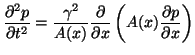 |
(1.21) |
which is sometimes called Webster's horn equation [15,30,66]. Due to the variation in the cross-sectional area, it is not equivalent to the one-dimensional wave equation (1.3), and does not possess a simple solution in terms of traveling waves (which is why we needed a concatenated uniform tube model in the first place).
Returning now to the DWN of Figure 1.4, it can be shown that the junction pressures
 (at spatial locations and at time for and integer) satisfy a recursion of the form
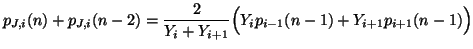 |
(1.22) |
where  is the admittance of the th acoustic tube, running from
 to . With the set according to (1.7), it is again possible to show that (1.22) is a finite difference scheme for (1.21), with
.
to . With the set according to (1.7), it is again possible to show that (1.22) is a finite difference scheme for (1.21), with
.
Next: A General Approach: Multidimensional
Up: Digital Waveguide Networks
Previous: Waveguide Meshes and the
Stefan Bilbao
2002-01-22