Next: Junctions Between Two Uniform
Up: Case Study: The Kelly-Lochbaum
Previous: Concatenated Acoustic Tube Model
The concatenated tube model is useful because the acoustic behavior of a single tube of constant cross-sectional area  is quite simple to describe, in terms of a volume velocity
  , and a pressure deviation
  from the mean tube pressure. Provided wavelengths are long in comparison with the tube radius, and that pressures do not become too large (both these requirements are easily satisfied in the speech context), the time-evolution of the acoustic state of any single tube, such as that shown in Figure 1.2(a), will be described completely by
 |
(1.1a) |
subject, of course, to initial conditions, and the effect of the boundary terminations on adjacent tubes. Given that the cross-sectional tube area , the air density  and the sound-speed
  are constant, the general solution to (1.1) can be written as
 |
(1.2a) |
Here the physical pressure  has been decomposed into a sum of a leftward-traveling wave
  and a rightward-traveling wave
  ; both are arbitrary functions of one variable. The volume velocity
  , which is dual to in the system (1.1), can be similarly expressed as a sum of leftward- and rightward-traveling velocity waves
  and
and  . But these velocity waves are simply the pressure waves, scaled by the tube admittance, defined by
In addition, the rightward-traveling wave component of the velocity is sign-inverted with respect to the corresponding pressure wave.
System (1.1) can be simplified to a single second-order PDE in pressure alone,
 |
(1.3) |
from which the traveling pressure wave solution is more easily extracted. The volume velocity satisfies an identical equation.
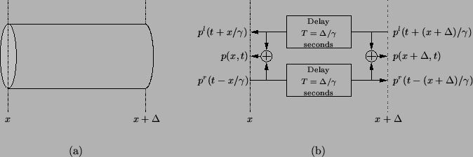
Consider one of the tube segments of length  from Figure 1.1(b). It should be clear that we can represent the pressure traveling-wave solution to (1.1) by using two delay lines, each of duration
 ; see Figure 1.2. We can obtain the physical pressure at either ends of the tube by summing the leftward- and rightward-traveling components, as per (1.2a). (The physical volume velocity can be obtained, from (1.2b), by taking the difference of and , and scaling the result by
  .) The discrete-time implementation of this single isolated acoustic tube is immediate. Taking
 |
(1.4) |
as the unit delay, or sampling period for our discrete-time system,
we can see that there is no loss in generality in treating the paired shifts as digital delay lines, accepting and shifting discrete-time pressure wave signals, at intervals of  seconds. The discrete-time model of the acoustic tube will still calculate an exact solution to system (1.1), at times which are integer multiples of . (This solution can be considered to be exact at all time instants as long as all signals in the network are assumed to be bandlimited to half of the sampling rate,
 .)
.)
Figure 1.2: (a) An acoustic tube and (b) a representation of the traveling wave solution; traveling pressure waves can be added together at either end of the tube to give the physical pressure, as per (1.2a).
|
|
Also note that because the traveling pressure and volume velocity waves are simply related to one another by a scaling, then in a computer implementation, it is only necessary to propagate one of the two types of wave in a given discrete tube section--we will assume, then, that pressure waves are our signal variables.
Next: Junctions Between Two Uniform
Up: Case Study: The Kelly-Lochbaum
Previous: Concatenated Acoustic Tube Model
Stefan Bilbao
2002-01-22