Next: Power Conservation at Scattering
Up: Case Study: The Kelly-Lochbaum
Previous: Wave Propagation in a
Consider now a junction between two of the uniform acoustic tubes in the concatenated tube model shown in Figure 1.1(b). The wave speeds in all the tubes are assumed to be constant, and equal to  , so that the discrete-time representation of any single tube will have the form of the pair of digital delay lines shown in Figure 1.2(b). At the junction between the
  th and
  th tubes (of cross-sectional areas
 and
and
 respectively), for
 , we will then have a pressure and a velocity on either side; we will write these pressure/velocity pairs as
 , and
, and
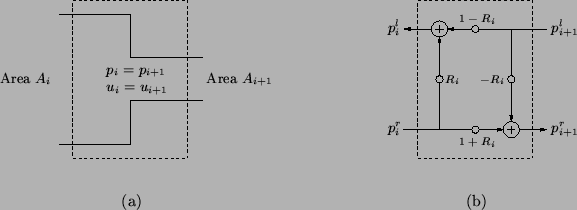
 respectively--see Figure 1.3(a). Continuity arguments (or conservation laws) dictate that these quantities should remain unchanged as we pass through the boundary between the two tubes, and thus
 |
(1.5) |
Note that we have dropped the arguments  and
and  , since the relationships of (1.5) hold instantaneously, and only at the tube boundaries.
Figure 1.3: (a) The junction between the th and th acoustic tubes in the Kelly-Lochbaum vocal tract model, and (b) the resulting scattering junction for pressure waves.
 |
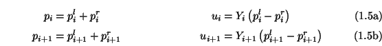
As per (1.2a) and (1.2b), the pressures and velocities can be split into leftward- and rightward-traveling waves as
where  , the admittance of the th tube, is defined by
 |
(1.7) |
It is then possible, using (1.6) to rewrite (1.5) purely in terms of the wave variables, as
 |
(1.8a) |
where
 is defined by
Here we have written a formula for calculating the pressure waves  and
and
 leaving the junction in terms of the waves
  and
and
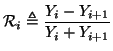
 entering the junction--see Figure 1.3(b) for the resulting signal-flow diagram. In particular, (1.8) can be viewed as a scattering operation; incident waves on either side of an interface are reflected and transmitted according to the mismatch in the admittances between the two tubes. The mismatch is characterized by the reflection parameter
which is bounded in magnitude by 1, as long as the admittances of the two tubes are positive. (If
entering the junction--see Figure 1.3(b) for the resulting signal-flow diagram. In particular, (1.8) can be viewed as a scattering operation; incident waves on either side of an interface are reflected and transmitted according to the mismatch in the admittances between the two tubes. The mismatch is characterized by the reflection parameter
which is bounded in magnitude by 1, as long as the admittances of the two tubes are positive. (If
 , for instance, then
 , and there is no reflection at the interface.) As we mentioned before, the calculations (1.8) should be viewed as occurring pointwise at the junction interface itself, which does not occupy physical space.
Suppose that we define a set of power-normalized wave variables by
 |
(1.9) |
Then the scattering operation (1.8) can be written, in matrix form, as
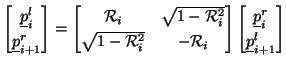 |
(1.10) |
Because the
are bounded in magnitude by 1, it is easy to see that scattering, in this case, corresponds to an orthogonal matrix transformation applied to the input wave variables.
Next: Power Conservation at Scattering
Up: Case Study: The Kelly-Lochbaum
Previous: Wave Propagation in a
Stefan Bilbao
2002-01-22