Digital Waveguide Networks

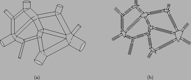
The principal components of the Kelly-Lochbaum speech synthesis model, paired delay lines which transport wave signals in opposite directions, and the scattering junctions to which they are connected, are the basic building blocks of digital waveguide networks (DWNs) [166]. Keeping within the acoustic tube framework, it should be clear that any interconnected network of uniform acoustic tubes can be immediately transferred to discrete time by modeling each tube as a pair of digital delay lines (or digital waveguide) with an admittance depending on its cross-sectional area. At a junction where several tubes meet, these waves are scattered. See Figure 1.6 for a representation of a portion of a network of acoustic tubes, and its DWN equivalent.

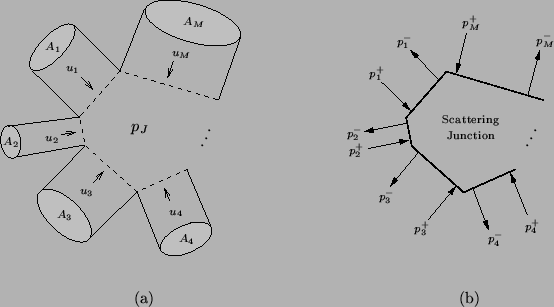
Figure 1.6: (a) A portion of a general network of one-dimensional acoustic tubes and (b) its discrete-time realization using paired bidirectional delay lines and scattering junctions.

The scattering operation performed on wave variables must be generalized to the case of the junction of $M$ tubes, as shown in Figure 1.7. Though we will cover this operation in more detail in Chapter 4, and in the wave digital context in Chapter 2, we note that as for the case of the junction between two tubes, the scattering equations result from continuity requirements on the pressures and volume velocities at the junction. That is, if the pressures in the $M$ tubes at the junction are $p_{j}$, and the velocities are $u_{j}$, $j=1,\hdots,M$ (we now fix the sign of $u_{j}$ to be positive if velocities are in the direction of the junction), then the relations are

In other words, the pressures in all the tubes are assumed to be identical and equal to some junction pressure $p_{J}$ at the junction, and the flows must sum to zero, by conservation of mass. These are the acoustic analogues of Kirchoff's Laws for a parallel connection of $M$ electrical circuit elements, where pressures are interpreted as voltages, and velocities as currents.

The pressures and velocities can be split into incident and reflected waves $p_{j}^{+}$ and $p_{j}^{-}$ as per (1.2a) and (1.2b), by

$$p_{j} = p_{j}^{+}+p_{j}^{-}\hspace{1.0in}u_{j} = Y_{j}\left(p_{j}^{+}-p_{j}^{-}\right)$$

where $Y_{j}$ is the admittance of the $j$th tube. The scattering relation, which can then be derived from (1.12), is

$$p_{k}^{-} = -p_{k}^{+} + \frac{2}{\sum_{j=1}^{M}Y_{j}}\sum_{j=1}^{M}Y_{j}p_{j}^{+}\hspace{1.0in}k=1,\hdots,M$$ (1.13)

and can be represented graphically as per Figure 1.7(b).

Figure 1.7: (a) A junction of $M$ acoustic tubes, indicating the pressures $p_{j}$ and volume velocities $u_{j}$ in the $j$th tube, $j=1,\hdots,M$ at the junction and (b) a scattering junction relating outgoing pressure waves $p_{j}^{-}$ to incoming waves $p_{j}^{+}$, $j=1,\hdots,M$.

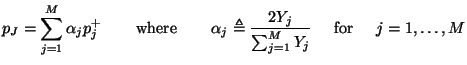
It is worth examining this key operation in a little more detail. First note that the scattering operation can be broken into two steps, as follows. First, calculate the junction pressure $p_{J}$, by

$$p_{J} = \sum_{j=1}^{M}\alpha_{j}p_{j}^{+}\hspace{0.3in}{\rm where... ...c{2Y_{j}}{\sum_{j=1}^{M}Y_{j}}\hspace{0.2in}{\rm for}\hspace{0.2in}j=1,\hdots,M$$ (1.14)

Then, calculate the outgoing waves from the incoming waves by

$$p_{k}^{-} = -p_{k}^{+} + p_{J}\hspace{1.0in}k=1,\hdots,M$$

Although (1.13) produces $M$ output waves from $M$ input waves, and can thus be written as an $M\times M$ matrix multiply, the number of operations is $O(M)$ ($M$ multiplies and 2$M-$1 adds). Also note that the physical junction pressure is calculated, from (1.14), as a natural by-product of the scattering operation; because in a numerical integration setting, this physical variable is always what we are ultimately after, we may immediately suspect some link with standard differencing methods, which operate exclusively using such physical ``grid variables''. In Chapter 4, we examine the relationship between finite difference methods and DWNs in some detail.

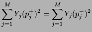
It is simple to show that the scattering operation also ensures that

$$\sum_{j=1}^{M}Y_{j}(p_{j}^{+})^{2} = \sum_{j=1}^{M}Y_{j}(p_{j}^{-})^{2}$$ (1.15)

which is, again, merely a restatement of the conservation of power at a scattering junction. Notice that if all the admittances are positive, then a weighted $L_{2}$ norm of the wave variables is preserved through the scattering operation. (If power-normalized variables are employed, then scattering is again equivalent to an $M\times M$ orthogonal matrix transformation.) The network as a whole will behave losslessly through the scattering and shifting operations which constitute a single step in the global recursion that such a network implies.