Relationship to Digital Filters

Discrete-time structures such as that shown in Figure 1.4 are also used in digital filtering applications [134,139], in which case, the notion of a spatial location associated with a particular junction or delay element is often lost. For example, consider the digital filter structure shown in Figure 1.5(a).

Figure 1.5: (a) An all-pole lattice filter, and (b) a standard lattice junction, (c) a Kelly-Lochbaum junction and (d) a normalized lattice junction.

With $x(n)$ as a real discrete-time input sequence indexed by integer $n$, and $y(n)$ as the output sequence, this structure is called an all-pole lattice filter [134], when any of the types of section shown in Figure1.5(b), (c) or (d) is used. $T$ is the sample period, or unit delay, and the structure is parameterized by the constants $k_{i}$, $i=1,\hdots,N$. It is possible to show that $x(n)$ and $y(n)$ are related by the familiar all-pole difference equation

$$y(n) = x(n) + \sum_{i=1}^{N}a_{i}y(n-i)$$ (1.11)

where the direct-form filter coefficients $a_{i}$, $i=1,\hdots,N$ can be derived from the $k_{i}$ through simple recursive procedures [134]. While the direct-form filter implementation implied by (1.11) requires fewer arithmetic operations than the lattice forms in Figure 1.5, the lattice implementation may be preferable because (a) stability is guaranteed by the simple condition $\vert k_{i}\vert< 1$, for all $i$, (determining stability by direct examination of the $a_{i}$ is difficult, though it can of course be performed by finding the equivalent set of $k_{i}$ parameters) and (b), pole locations are much less sensitive to coefficient quantization when applied to the $k_{i}$ rather than the $a_{i}$. We also mention that the same structure also doubles as a useful all-pass filter design [134], when $x(n)$ is taken as the input and $w(n)$ as the output. It is also possible to extend this filter design in order to implement any general stable pole-zero filter by summing readout taps from the leftward signal path into the output [139].

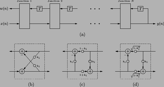The structure of Figure 1.5(a) is quite similar to the Kelly-Lochbaum discrete-time acoustic tube model, but there are two minor differences. First, the Kelly-Lochbaum structure contains delay elements in both the leftward and rightward signal paths, reflecting the traveling-wave nature of the solution to the physical acoustic tube problem. In the lattice filter structure, however, the delays all occur in the upper (leftward) signal path. It is possible to transform the Kelly-Lochbaum structure into the lattice form by signal flow-graph manipulations involving pushing delays through the junctions, combining them, and then downsampling by a factor of two--this can be done provided the acoustic tube model is terminated by a zero or infinite impedance at the right end [166]. (We remark that this downsampling operation can also be applied to digital waveguide meshes in higher dimensions, in which case we will refer to it as grid decimation; we will examine grid decimation for a variety of mesh forms in Appendix A.) Second, the Kelly-Lochbaum and normalized junctions in our treatment of the acoustic tube model differ slightly from the signal flow graphs shown in Figure 1.5(c) and (d). This difference is due to our choice of pressure waves instead of velocity waves as our signal set. While these quantities are dual in the one-dimensional acoustic tube, this symmetry is lost when we move to acoustics problems in higher dimensions, and it is more natural to work with pressure variables.

The same lattice structure is also arrived at in the analysis context when linear predictive coding (LPC) techniques are applied to a speech waveform [124]. The assumption underlying LPC is that speech can be treated as a source signal (such as a glottal waveform), filtered by the vocal tract, and the goal is to design an all-pole filter of the form of (1.11) which models the system resonances (or formant structure). Though this filter is obtained through purely autoregressive (i.e., non-physical) analysis of a given measured speech signal, the reflection coefficients $k_{i}$ (also known as partial correlation or PARCOR coefficients) are calculated as a byproduct of the main calculation of the direct form filter coefficients $a_{i}$. The $k_{i}$ are identical to the $\mathcal{R}_{i}$ in the acoustic tube model, except for a sign inversion. This is not to say that the filter arrived at through LPC immediately implies a particular vocal-tract shape; it is best thought of as the solution to a filter-design or system identification problem, devoid of any physical interpretation [145]. We note, though, that transmission-line models such as the concatenated acoustic tube model have long been used for such system identification purposes in the inverse scattering context, in which case they are sometimes referred to as ``layer-peeling'' or ``layer-adjoining'' methods [22,23,213]. Provided certain assumptions are made about the glottal waveform and the effects of radiation on the measured speech waveform, it is possible to make some inferences about the vocal tract shape [30].