Discrete-time Vocal Tract Model

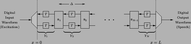
Now that we have discussed both the digital delay line representation of wave propagation within a single acoustic tube, as well as the scattering that occurs at any junction between adjacent tubes, we are now ready to present the full discrete-time model of the vocal tract. For an $N$ tube model of the vocal tract, then, we will have the digital signal flow graph shown in Figure 1.4. Here, the scattering junctions are indicated by rectangles, marked by ${\bf S}_{i}$ (representing a matrix transformation of the form of (1.8) or (1.10), which is parametrized by $\mathcal{R}_{i}$, which itself depends on the adjoining tube admittances $Y_{i}$ and $Y_{i+1}$).

Figure 1.4: Signal flow graph for an $N$ tube vocal tract model.

The structure is driven at the left end, by an input waveform (typically an impulse train, for voiced speech or by white noise for unvoiced speech, or a combination of the two), and an output speech waveform is emitted at the right end. The grey boxes, representing boundary conditions at the glottis and lips, we leave unspecified--such terminations can be modeled in a variety of ways [145].

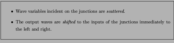
Leaving aside a discussion of these boundaries, we can see that a single cycle in the recursive structure shown in Figure 1.4 (one pass through the main loop of the computer program that it implies) will involve two distinct steps:

We have already seen that the scattering operation preserves a weighted $L_{2}$ norm of the signal variables; it should be obvious that the shifting operation also does so, trivially (indeed, in the computer program, shifting amounts to no more than a permutation of the set of pressure signals stored in memory). Thus we have a simple positive definite measure of the state of the tube in terms of signal values stored in the delay registers which remains constant as time progresses (again, excepting the effect of the boundary conditions). What is more, this numerical stability property of this structure is very easy to verify; we need only check that all the reflection coefficients $\mathcal{R}_{i}$ are bounded by 1 in magnitude, or equivalently, that all the admittances are positive. The excitation at the left boundary will, of course, introduce energy into the system, but we can at least be sure that signal energy is not being produced in the problem interior. The energy drain at the radiating (right) boundary is similarly localized.

Several other features are worthy of comment. First, we have treated the vocal tract here as a static or time-invariant linear (LTI) system. As we mentioned before, however, the configuration of the vocal tract must necessarily change during any utterance--these variations are assumed to be slow with respect to the frequency content of the excitation. The slow variation in the acoustic tube profile will cause shifts in the system resonances (formants), and these shifts will be perceived, by the listener, as phoneme transitions. In our discussion of scattering and energy conservation in the Kelly-Lochbaum model, we have not taken the time variation of the tube cross-sectional areas (and thus the reflection coefficients) into account. It should be clear, though, that if we are using the power-normalized signal variables defined by (1.9), then scattering defined by (1.10) at any junction remains an orthogonal (and thus norm preserving) operation, even if the $\mathcal{R}_{i}$ are functions of time [166]. Second, it is also simple to extend the model to include the nasal pathways (necessary for the production of certain vocal sounds, and also modeled as acoustic tubes [30]), without compromising overall losslessness. Third, we note that the stability of this model can be maintained even if the reflection coefficients $\mathcal{R}_{i}$ are quantized [166]--this will necessarily occur in any finite word-length machine implementation. As long as the quantized coefficients remain bounded by 1, then we still have a perfectly lossless system. Signal quantization can also be performed so as to maintain overall stability, though the system will become more generally passive and not strictly lossless. Fourth, although the acoustic tube of varying cross-sectional area is often considered to be analogous to a lossless electrical transmission line of spatially-varying inductance and capacitance, it is better thought of as a special case of the latter. For the acoustic tube, the local admittance varies directly with the cross-sectional area, but the wave speed $\gamma$ remains constant; this is important, because for a given tube length of $\Delta$, the time delay is dependent on the wave speed, from (1.4). For a transmission line, both the admittance and the wave speed may vary from point to point along its length. We cannot then approximate the full transmission line by concatenated uniform transmission line segments in the same way as for the acoustic tube without losing synchronization of the resulting discrete-time structure (i.e., delay durations in the segments are not all the same). We will show how to solve this problem in Chapter 4.