A General Approach: Multidimensional Circuit Representations and Wave Digital Filters

For the Kelly-Lochbaum vocal tract model, it is straightforward to arrive at a numerical scattering formulation of the problem; the approximation of a smoothly-varying tube by a series of concatenated tubes is intuitively satisfying, and leads immediately to a wave variable numerical solution to Webster's equation. The identification of the mesh of one-dimensional tubes of Figure 1.8(a) as a numerical solver for the two-dimensional wave equation is more difficult, because it is by no means clear that such a mesh behaves like a two-dimensional acoustic medium (say). Although as we have seen, it is possible to prove (through a finite difference treatment) that the tube network is indeed solving the right equation, we have not shown a way of deducing such a structure from the original defining PDE system. If one wants to develop a DWN for a more complex system (such as a stiff vibrating plate of variable density and thickness, for example), then guesswork and attempts at invoking Huygens' principle will be of limited use.

The scattering operation we introduced in §1.1.1 and §1.1.2 is at the heart of all the numerical methods we will discuss in this thesis, whether they are based on digital waveguide networks or wave digital filters, which we will shortly introduce. A given system of PDEs is numerically solved by filling the problem domain with scattering nodes, or junctions, such as that shown in Figure 1.7(b), which calculate reflected waves from incident waves according to (1.13) (or its series dual form). The topology of the network of interconnected junctions will be dependent on the particulars of the system we wish to solve. As we have seen, these scattering junctions act as power-conserving signal processing blocks, and in a DWN, they are linked by discrete-time acoustic tubes, or transmission lines, which are also power-conserving, and serve to transport energy from one part of the network to another. The key concept here is the losslessness of the network components, which is dependent on the positivity of the various circuit element values (admittances); as we have seen, this positivity condition ensures that some squared norm of the signals in the discrete-time network will remain constant as time progresses. In other words, the simulation routine that such a network implies is guaranteed stable by enforcing this condition.

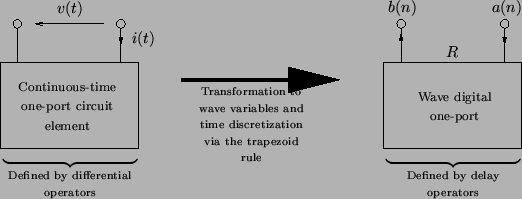
Wave digital filters (WDFs) are also based on the idea of preserving losslessness (and more generally passivity) in a discrete-time simulation of a physical system, though the approach is somewhat different from what we have just seen. As they were originally intended to transfer analog electrical filter (RLC) networks to discrete time, it is best to begin by looking briefly at lumped circuit elements. A one-port element, such as that shown at left in Figure 1.9 is characterized by a voltage $v$, and a current $i$, both of which are functions of time $t$. In the time domain, the one-port generally relates $v(t)$ and $i(t)$ through some combination of differential or integral operators. If the one-port (or more generally, $N$-port) is linear and time-invariant, then there is a simple description of its behavior in the frequency domain, but we will wait until Chapter 2 before entering into the details. An analog filter is simply an interconnected network of such elements; it is operated by applying a voltage at one pair of free terminals, and then reading the filtered output at another pair. In particular, if the network is made up of passive elements such as resistors, capacitors, inductors etc., then it must behave as a stable filter.

Figure 1.9: Wave digital discretization of a one-port circuit element.

Fettweis [46] developed a procedure for mimicking the energetic behavior of an analog filtering network in discrete time. The input and filtered output become digital signals, and the filtering network becomes a recursion, to be realized as a computer program. Most importantly, the digital network has the same topology as the analog network, and can be thought of as its discrete-time ``image.'' One-ports (or more generally $N$-ports) are first characterized in terms of wave variables,

$$a = v+iR$$

$$b = v-iR$$

where $R$ is some arbitrary positive constant, assigned to the particular one-port, called a port resistance. The continuous-time element, described by differential operators, is then replaced by a discrete-time element operating on digital signals, and composed of algebraic operations and delay operators or shifts. The signal $a(n)$ is called the input wave, and $b(n)$ is the output wave; both are discrete-time sequences indexed by integer $n$. If the discretization procedure is carried out in an appropriate way (to be more precise, differentiation is approximated by the trapezoid rule of numerical integration), then the resulting wave digital one-port has energetic properties very similar to the continuous element from which it is derived. In particular, if the analog element is passive (lossless), then the wave digital element can be considered to passive (lossless) in a similar sense. In fact, if a wave digital circuit element is composed of delay operators (hence requiring memory), then a weighted sum of the squares of the signal values stored in the element's delay registers is the direct counterpart to the physical energy stored in the electric and magnetic fields surrounding the corresponding analog element. The passivity property is contingent on the positivity of the port resistance; given this constraint, it can often be chosen such that there is no delay-free path from the input $a(n)$ to the output $b(n)$. We will see the importance of making the correct choice of $R$ shortly in an example.

Figure 1.10: (a) Parallel connection of two continuous-time one-ports and (b) its wave digital counterpart.

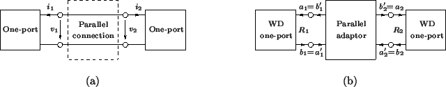
Consider a parallel connection of two one-port circuit elements, as shown in Figure 1.10(a). The one-ports are defined by some relationship between their respective voltages and currents, which we will write as $v_{1}$, $i_{1}$ and $v_{2}$, $i_{2}$. For such a parallel connection, Kirchoff's Laws dictate that

$$v_{1} = v_{2}\hspace{1.5in}i_{1}+i_{2} = 0$$ (1.23)

(We could equally well treat this as a series connection, by reversing the directions of the arrows which define $v_{2}$ and $i_{2}$ in Figure 1.10(a).) We can now define two sets of wave variables at the two one-ports by

$$a_{1} = v_{1} + i_{1}R_{1}\hspace{1.5in}a_{2} = v_{2} + i_{2}R_{2}$$

$$b_{1} = v_{1} - i_{1}R_{1}\hspace{1.5in}b_{2} = v_{2} - i_{2}R_{2}$$

In the scattering formulation, the Kirchoff connection is treated as a separate two-port element, with inputs $a_{1}'$ and $a_{2}'$ and outputs $b_{1}'$ and $b_{2}'$. These are simply the outputs and inputs, respectively, of the one-ports, as shown in Figure 1.10(b).

Kirchoff's Laws for the parallel connection can then be rewritten in terms of the wave variables as

$$\begin{eqnarray}b_{1}' &=& \mathcal{R}a_{1}' + (1-\mathcal{R})a_{1}'\\ b_{2}' &=& (1+\mathcal{R})a_{1}'-\mathcal{R}a_{2}' \end{eqnarray}$$ (1.24a)

where the reflection coefficient $\mathcal{R}$ is defined by

$$\mathcal{R} \triangleq \frac{R_{2}-R_{1}}{R_{2}+R_{1}}$$

Equations (1.24) define a wave digital two-port parallel adaptor. They are identical in form to the equations defining a parallel junction of two acoustic tubes, from (1.8)--this is to be expected, since Kirchoff's Laws (1.23) are equivalent to the pointwise continuity equations (1.5) at an acoustic junction. Thus all comments we made about scattering junctions in §1.1.1 hold for the wave digital adaptor as well; in particular, if we define power-normalized waves, then the scattering operation again is equivalent to an orthogonal (i.e., $L_{2}$ norm-preserving) transformation, as long as the port resistances $R_{1}$ and $R_{2}$ are chosen positive (implying, again, that $\vert\mathcal{R}\vert<1$).