An Interleaved Waveguide Network

The simplified waveguide network described above solves the wave equation for voltage, at the magic time step, $T = \Delta/\gamma$. That is, the junction voltages $U_{J}$ solve the difference equation (4.24), and hence approximate $u$. We would, however, like to be able to have direct access to a discrete equivalent of the other variable as well, the current $i$.

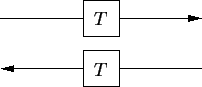
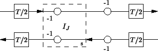
Bearing in mind the discussion in §4.3.2 on interleaved grids, examine the identity pictured in Figures 4.10 and 4.11.

Figure 4.10: Bidirectional delay line.

Figure 4.11: Split equivalent to the bidirectional delay line.

We have merely split the unit sample bidirectional delay line into two half-sample delay lines of equal impedance, and placed a series junction (in cascade with sign inverters) in between. In this case, since there is no scattering, the net behavior of the junction and sign inversion is that of a simple ``through,'' with sign inversions exactly canceling those that appear in the signal path (these can be added formally using transformers). Later we will add additional ports to this new junction. We introduce these series junctions so as to be able to associate a junction current with them, which we will identify with the physical current in the transmission line.

If we now replace all the bidirectional delay lines in Figure 4.8 by the split pair of lines, then we get the arrangement in Figure 4.12.

Figure 4.12: (1+1)D interleaved waveguide network.

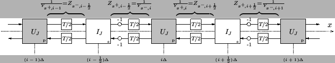As at the parallel junctions, we can define wave voltages and currents at the series junctions, which we will index by $i+\frac{1}{2}$ for $i$ integer. Furthermore, we name the impedances at the left- and right-hand ports of the series junctions $Z_{x^{-},i-\frac{1}{2}}$ and $Z_{x^{+},i-\frac{1}{2}}$ respectively. As indicated in Figure 4.12, we must also have

$$Z_{x^{+},i-\frac{1}{2}} = \frac{1}{Y_{x^{-},i}}\hspace{0.5in}Z_{x^{-},i+\frac{1}{2}} = \frac{1}{Y_{x^{+},i}}$$

The junction impedance at the series junctions will be

$$Z_{J,i+\frac{1}{2}} \triangleq Z_{x^{-},i+\frac{1}{2}}+Z_{x^{+},i+\frac{1}{2}} = \frac{1}{Y_{x^{+},i}}+\frac{1}{Y_{x^{-},i+1}}$$

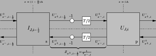
See Figure 4.13 for a complete picture of the various wave quantities at the interleaved junctions.

Figure 4.13: Wave quantities in the interleaved network of Figure 4.12.

Assuming that the impedances in all the delay lines are identical and equal to $Z$ (and so $Z_{J,i-\frac{1}{2}}=2Z$), we can now define

$$I_{J,i-\frac{1}{2}} = \frac{2}{Z_{J,i-\frac{1}{2}}}\left(Z_{x^{+},i-\frac{1}{2}}I_{x^{+},i-\frac{1}{2}}^{+}+Z_{x^{-},i-\frac{1}{2}}I_{x^{-},i-\frac{1}{2}}^{+}\right)$$

$$= I_{x^{+},i-\frac{1}{2}}^{+}+I_{x^{-},i-\frac{1}{2}}^{+}$$

We also have that

$$U_{x^{-},i}^{+}(n) = -U_{x^{+},i-\frac{1}{2}}^{-}(n-{\textstyle \frac{1}{2}})$$

$$U_{x^{+},i-\frac{1}{2}}^{+}(n+{\textstyle \frac{1}{2}}) = -U_{x^{-},i}^{-}(n)$$

and (4.26) holds as before.

We now show that this waveguide network performs a calculation identical to that which we would get for centered differences on a decimated grid, exactly as in Figure 4.7. For integer $i$ and $n$, we have:

$$U_{J,i}(n)\hspace{0.1in} = U_{x^{+},i}^{+}(n)+U_{x^{-},i}^{+}(n)$$

$$= Z\left(I_{x^{+},i}^{+}(n)+I_{x^{-},i}^{+}(n)\right)$$

$$= - Z\left(I_{x^{-},i+\frac{1}{2}}^{-}(n-{\textstyle \frac{1}{2}})-I_{x^{+},i-\frac{1}{2}}^{-}(n-{\textstyle \frac{1}{2}})\right)$$

$$= - Z\left(I_{J,i+\frac{1}{2}}(n-{\textstyle \frac{1}{2}})-I_{J,i-\frac{1}{2}}(n-{\textstyle \frac{1}{2}})\right)$$

$$\hspace{0.5in}+\hspace{0.1in}Z\left(I_{x^{-},i+\frac{1}{2}}^{+}(n... ...le \frac{1}{2}})-I_{x^{+},i-\frac{1}{2}}^{+}(n-{\textstyle \frac{1}{2}})\right)$$

$$= - Z\left(I_{J,i+\frac{1}{2}}(n-{\textstyle \frac{1}{2}})-I_{J,i-\frac{1}{2}}(n-{\textstyle \frac{1}{2}})\right)$$

$$\hspace{0.5in}+\hspace{0.1in} U_{x^{+},i}^{-}(n-1)+U_{x^{-},i}^{-}(n-1)$$

$$= - Z\left(I_{J,i+\frac{1}{2}}(n-{\textstyle \frac{1}{2}})-I_{J,i-\frac{1}{2}}(n-{\textstyle \frac{1}{2}})\right)+ U_{J,i}(n-1)$$ (4.35)

If we now identify $I_{J}$ with $I$ and $U_{J}$ with $U$, we get (4.22b) (in the constant-coefficient case), with $Z = 1/(v_{0} c)$. A similar derivation beginning from the series (white, in Figure 4.12) junctions yields (4.22a), with $Z = v_{0}l$, for constant $l$. Together, these constraints imply that:

$$v_{0} = \frac{1}{\sqrt{lc}}\hspace{0.5in}Z = \sqrt{\frac{l}{c}}$$

so that we are again at the magic time step. Furthermore, the impedance of any waveguide in the network must be set equal to the characteristic impedance of the continuous time/space transmission line described by (4.17), whereas in the network of Figure 4.8, the constant impedance value could be set arbitrarily, since it is not used in the simulation. It is important to realize that, at least in this constant-coefficient case, no scattering occurs at any of the junctions. We can still perform all operations at the original sampling rate, and on the original grid (i.e., with grid spacing $\Delta$ and time step $T$). It is, however, possible to see more clearly how initial (and boundary) conditions must be set, and also to extend the network to handle more complex problems. We will deal with one such generalization in the next section.