Next: Type III: Mixed Network
Up: Varying Coefficients
Previous: Type I: Voltage-centered Network
This arrangement is the dual to the previous case. We now set
and
 |
(4.49) |
We have thus chosen
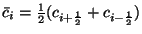 and
and
 .
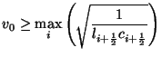
Now we must have
.
Now we must have
which is very similar to condition (4.36), except that the maximum is now taken over the series junction locations.
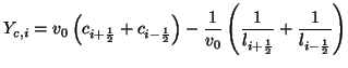
Here, scattering at the series junctions is trivial, since the impedances at the two connecting ports are identical, and the self-loop impedance is zero (and we thus drop entirely any calculation of the value in the self-loop at the series nodes). We can operate at the down-sampled rate, with scattering occurring only at the parallel junctions. In this case, we are directly computing only junction voltages, and are in fact solving the second-order reduction of system (4.17), namely
 |
(4.50) |
We could have made a similar statement about scattering at the parallel junctions in the previous case. This efficient configuration, unlike type I, however, generalizes to the (2+1)D case, as we will see in §4.4.2.
Next: Type III: Mixed Network
Up: Varying Coefficients
Previous: Type I: Voltage-centered Network
Stefan Bilbao
2002-01-22