Next: Phase and Group Velocity
Up: Multidimensional Wave Digital Filters
Previous: Simplified Networks
The (2+1)D Parallel-plate System
Generalizing the above procedure to several dimensions is straightforward. We examine here, as a practical example, the (2+1)D parallel-plate system, which is written as:
 |
(3.63a) |
This system was treated using MDWDFs in [62,211].
Now the dependent variables are a voltage  , and current density components
  and
and  ; these, and the sources
  ,
,  and
and  are functions of time
  and two spatial variables,
  and
and  .
.  ,
,  ,
,  and
and  are arbitrary smooth positive functions of and ( and are strictly positive). It is worth mentioning that the same equations can be used in the contexts of (2+1)D linear acoustics, the vibration of a membrane, and, with a trivial modification, (2+1)D electromagnetic field problems (involving TE or TM modes).
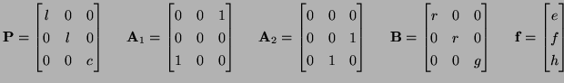
System (3.67) is symmetric hyperbolic, and thus has the form of (3.1), where
![$ {\bf w} = [i_{x}, i_{y}, u]^{T}$](img856.png) , and with
, and with
It will follow, as in the case of the (1+1)D transmission line system (see §3.7.4), that the total energy of the MDKC that we will derive in the next section will be equal to the energy of system (3.67), as per (3.6).
Subsections
Next: Phase and Group Velocity
Up: Multidimensional Wave Digital Filters
Previous: Simplified Networks
Stefan Bilbao
2002-01-22