Next: MDKC and MDWD Network
Up: The (2+1)D Parallel-plate System
Previous: The (2+1)D Parallel-plate System
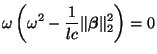
For the constant-coefficient, lossless and source-free case (i.e.,
 ), the numerical dispersion relation, in terms of the frequency
  and wavenumber magnitude


 will be, from (3.10),
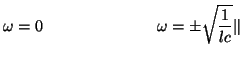
which has roots
Discounting the stationary mode with  , the phase and group velocities are then, from (3.12),
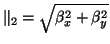
and if  and
and  are functions of
  and
and  , the maximal group velocity will be
 |
(3.64) |
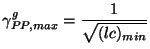
where
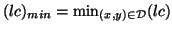 . This bound is the same as for the (1+1)D transmission line equations.
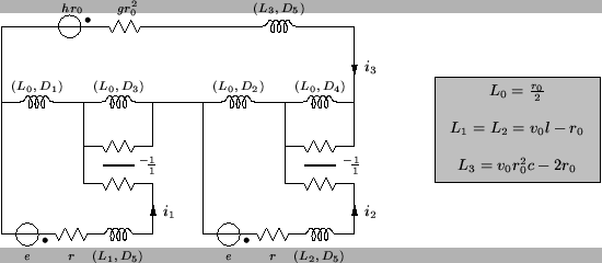
Figure 3.17:
MDKC for the (2+1)D parallel-plate system in rectangular coordinates.
|
|
Next: MDKC and MDWD Network
Up: The (2+1)D Parallel-plate System
Previous: The (2+1)D Parallel-plate System
Stefan Bilbao
2002-01-22