Because the stability of an explicit numerical method (such as those that we will examine in the rest of this thesis) which solves a system of hyperbolic equations is dependent on propagation velocities, it is worthwhile to spend a few moments here to define phase and group velocities [35,101] for a system such as (3.1).
Let us return to the unbounded domain problem with
![]() . Suppose that the matrices
. Suppose that the matrices ![]() ,
, ![]() and
and
![]() ,
,
![]() which define system (3.1) are real constants; in particular, we assume that the driving term
which define system (3.1) are real constants; in particular, we assume that the driving term ![]() is zero, and that
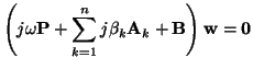
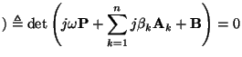
is zero, and that ![]() is anti-symmetric, so that system (3.1) is lossless. This is then a linear and shift-invariant system, and the solution can be written as a superposition of plane wave solutions of the form
is anti-symmetric, so that system (3.1) is lossless. This is then a linear and shift-invariant system, and the solution can be written as a superposition of plane wave solutions of the form
All the linear systems to be examined in this thesis are isotropic; propagation characteristics are independent of direction (though not necessarily of location, or frequency). For LSI systems, this implies that the dispersion relations (3.11) can be written as functions of
![]()
![]()
![]() alone, where
alone, where
![]()
![]()
![]() is simply the Euclidean norm of the vector
is simply the Euclidean norm of the vector
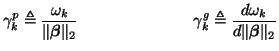
![]() . In this case, we may define the phase and group velocities for the
. In this case, we may define the phase and group velocities for the ![]() th relation by
th relation by
In the interest of extending these ideas to spatially inhomogeneous systems (of the form of (3.1) where ![]() and
and ![]() may exhibit a smooth functional dependence on
may exhibit a smooth functional dependence on
![]() ), we note that about any location
), we note that about any location
![]() , solutions to system (3.1) behave locally as solutions to the frozen-coefficient system [82] defined by
, solutions to system (3.1) behave locally as solutions to the frozen-coefficient system [82] defined by
![]() and
and
![]() . We may then define local group velocities
. We may then define local group velocities
![]()
![]()
![]() ,
,
![]() in the same way as in (3.12). A quantity which will appear frequently in our subsequent treatment of the stability of numerical methods for these systems will be the maximum global group velocity, defined as
in the same way as in (3.12). A quantity which will appear frequently in our subsequent treatment of the stability of numerical methods for these systems will be the maximum global group velocity, defined as
![$\displaystyle \gamma_{max}^{g} \triangleq \max_{\begin{minipage}[t]{1.0in}\vspa...
...d{minipage}}\gamma_{k}^{g}(\Vert\mbox{\boldmath$\beta$}\Vert _{2}, {\bf x}_{0})$](img534.png)