In a distributed problem, the dependent variables are functions not only of time ![]() , but also of location within an
, but also of location within an ![]() -dimensional spatial domain
-dimensional spatial domain
![]() , with coordinates
, with coordinates
![]() . Such a problem is referred to as an
. Such a problem is referred to as an ![]() D problem in the WDF literature [131]. Problems without spatial dependence will be called lumped problems. If the equations which define the problem include differential operators, we are faced with solving a set of partial differential equations (PDEs).
D problem in the WDF literature [131]. Problems without spatial dependence will be called lumped problems. If the equations which define the problem include differential operators, we are faced with solving a set of partial differential equations (PDEs).
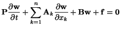
A particularly important family of PDE systems are the symmetric hyperbolic [74,82] systems of the form
Though it is possible to extend this definition to include cases where the matrices
![]() may depend on
may depend on ![]() ,
, ![]() or even
or even ![]() (in which case system (3.1) is nonlinear), this simpler form describes a wide variety of physical systems, from electromagnetics to string, membrane, beam, plate, shell, and elastic solid dynamics, to transmission line systems, to linear acoustics, etc. Symmetric hyperbolic systems are important because they form a subclass of strongly hyperbolic systems, for which the initial-value problem is well-posed [176]. Roughly speaking, to say that a system is well-posed is to say that the growth of its solution is bounded in a well-defined way; growth in an
(in which case system (3.1) is nonlinear), this simpler form describes a wide variety of physical systems, from electromagnetics to string, membrane, beam, plate, shell, and elastic solid dynamics, to transmission line systems, to linear acoustics, etc. Symmetric hyperbolic systems are important because they form a subclass of strongly hyperbolic systems, for which the initial-value problem is well-posed [176]. Roughly speaking, to say that a system is well-posed is to say that the growth of its solution is bounded in a well-defined way; growth in an ![]() norm cannot be faster than exponential. This concept is elaborated in detail in [82,176]. We can examine this growth in the present case as follows.
norm cannot be faster than exponential. This concept is elaborated in detail in [82,176]. We can examine this growth in the present case as follows.
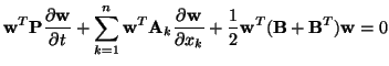
First, assume that the problem is defined over an unbounded spatial domain
![]() , so that we can drop any consideration of boundary conditions, and also that the forcing function
, so that we can drop any consideration of boundary conditions, and also that the forcing function
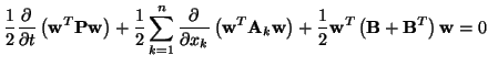
![]() . We now take the inner product of
. We now take the inner product of
![]() (the transpose of
(the transpose of ![]() ) with (3.1) to get
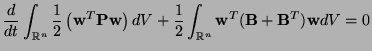
) with (3.1) to get
 |
In the MD circuit models that we will discuss, what we will be doing, in essence, is dividing this energy up among various reactive MD circuit elements. We will elaborate on this in the sections on the (1+1)D transmission line and (2+1)D parallel-plate system. The passivity condition is essentially equivalent to (3.7). Also, the symmetric nature of the systems will be reflected, in the circuit models, by the use of mainly reciprocal [12] circuit elements, though non-reciprocal elements (gyrators) will come into play if ![]() is not symmetric (it is not required to be, and note that system (3.1) is well-posed regardless of the form of
is not symmetric (it is not required to be, and note that system (3.1) is well-posed regardless of the form of ![]() [82]). We have not explored the application of passive circuit methods to systems which are more generally strongly hyperbolic, for which energy estimates such as (3.7) can also be derived [82]. This would appear to be a worthy direction of future research.
[82]). We have not explored the application of passive circuit methods to systems which are more generally strongly hyperbolic, for which energy estimates such as (3.7) can also be derived [82]. This would appear to be a worthy direction of future research.