MDKC and MDWD Network

The circuit can be derived along the same lines as for the (1+1)D case; we deal here with the discretization on a rectilinear grid, and will thus apply coordinate transformation defined by the ${\bf H}$ of (3.22). Rewriting system (3.67) in terms of the new coordinates $[t_{1},\hdots, t_{5}]^{T}$ using ${\bf\nabla_{u}} = {\bf VH}^{-R}{\bf\nabla_{t}}$, with the pseudo inverse (3.23) gives

$$\begin{eqnarray}\left(v_{0}l-r_{0}\right)D_{5}i_{1}&&\hspace{-0.2... ..._{0}}{2}D_{4}\left(i_{3}-i_{2}\right)+gr_{0}^{2}i_{3}+hr_{0} = 0 \end{eqnarray}$$

where we have used the new current-like variables

$$i_{1} \triangleq i_{x}\hspace{0.5in}i_{2} \triangleq i_{y}\hspace{0.5in} i_{3} \triangleq \frac{u}{r_{0}}$$

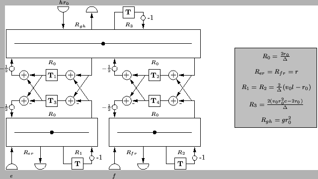
and $r_{0}$ is, as in the (1+1)D case, an arbitrary positive constant (which has also been used to scale (3.69c)). $D_{5} = D_{t'}$ will be treated as a simple time derivative, according to the generalized trapezoid rule discussed in §3.5.1. Figure 3.17 shows the MDKC that results from the transformed set of equations (3.69). The MDWD network corresponding to the MDKC is shown in Figure 3.18, where we have used step-sizes $T_{j} = \Delta$, $j=1,\hdots,5$.

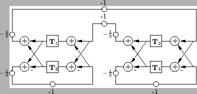
Figure 3.18: MDWD network for the (2+1)D parallel-plate system, in rectangular coordinates.

Passivity follows from a positivity condition on the network inductances, in particular $L_{1}$, $L_{2}$ and $L_{3}$ (the values of which are given in Figure 3.17). These conditions are

$$v_{0}\geq \frac{r_{0}}{l_{min}}\hspace{1.0in}v_{0}\geq\frac{2}{r_{0}c_{min}}$$ (3.66)

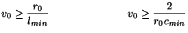
The choice of $r_{0} = \sqrt{\frac{2l_{min}}{c_{min}}}$, where $l_{min} = \min_{x,y}l$ and $c_{min} = \min_{x,y}c$ gives a stability bound of

$$v_{0}\geq\sqrt{\frac{2}{l_{min}c_{min}}}\geq \sqrt{2}\gamma_{PP,max}^{g}$$ (3.67)

which is the best possible bound for this network [61]. Note that $v_{0}$ is again bounded away from the maximum group velocity, even taking into account the scaling factor ($\sqrt{2}$ in this case), which is a consistent feature of explicit numerical methods in multiple spatial dimensions.

If $l$ and $c$ are constant, and in addition $r$, $g$, $e$, $f$ and $h$ are zero, and (3.71) holds with equality, i.e., we have

$$v_{0} = \sqrt{2}\gamma_{PP,max}^{g}$$ (3.68)

then the network of Figure 3.18 simplifies to the structure shown in Figure 3.19. This particular structure bears a very strong resemblance to the (2+1)D waveguide mesh [157,198] which we saw briefly in §1.1.2, and will examine in detail in Chapter 4.

Figure 3.19: Simplified MDWD network for the (2+1)D transmission line equations, in the lossless, source-free and constant parameter case.