


Next: MD-passivity
Up: Coordinate Changes in Higher
Previous: Coordinate Changes in Higher
Embeddings
In order to obtain a standard rectilinear grid in higher dimensions, it is possible to proceed in the same fashion, but it is in fact more convenient to extend the class of coordinate transformations so as to embed the problem domain in a higher dimensional space. In [62], the following generalization of (3.15) has been put forth:
 |
(3.20a) |
Here,  is still the
  -dimensional vector
![$ [x_{1},\hdots, x_{n},t]^{T}$](img570.png) , but
, but  is
is  -dimensional, with
  .
.  must be chosen such that the elements in its bottom row are positive.
 is a
is a
 right pseudo-inverse [92] of
 --in order to satisfy a generalization of the first of conditions (3.14), it must be chosen so that the elements in its rightmost column are all positive.
For example, for a (2+1)D problem with
--in order to satisfy a generalization of the first of conditions (3.14), it must be chosen so that the elements in its rightmost column are all positive.
For example, for a (2+1)D problem with
![$ \mathbf{u}=[x,y,t]^{T}$](img575.png) , in order to generate a rectilinear grid, the following choice is usually made:
, in order to generate a rectilinear grid, the following choice is usually made:
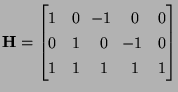 |
(3.21) |
projects five-dimensional coordinates
![$ \mathbf{t} = [t_{1},t_{2},t_{3},t_{4},t_{5}]^{T}$](img577.png) back to the three-dimensional space of .
One choice [62] for this right pseudo-inverse is
back to the three-dimensional space of .
One choice [62] for this right pseudo-inverse is
  |
(3.22) |
Uniform sampling in the coordinates, with step sizes of
 ,
,
 yields the standard rectangular grid shown in Figure 3.2(b), which is a pattern equivalent to what one would get by sampling uniformly (see comment below) in the
 coordinates, with a spacing of
  in all three untransformed variables. It should be clear that to every grid point in the coordinates corresponds a two-parameter family of points in the coordinates; this fact will not influence the resulting difference schemes. This embedding of the problem domain in a higher dimensional space is simply a means to an end; in particular, we will not be solving a system numerically over a higher-dimensional grid (which would be computationally infeasible). The new coordinate directions are chosen so that they define a grid, and they will also serve as directions of energy flow for the MD circuit elements which we will define presently. In effect, the total energy flow in a physical system is broken up among these new coordinate directions; it will sometimes be true (as in the case of a rectilinear grid in (2+1)D) that energy can approach a particular grid location from a number of neighbors which is greater than the dimensionality of the problem (for the (2+1)D parallel-plate problem on a rectilinear grid, at least four: north, south, east and west). We will take a closer a look at this particular transformation, its suitability for calculation on a rectilinear grid in §3.8.
In (3+1)D, in order to obtain a standard rectilinear sampling pattern, Nitsche has proposed seven-dimensional coordinates [62] defined by
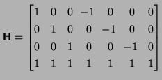 |
(3.23) |
It is easy to verify that shifts of distance along the coordinates  ,
,
 correspond to shifts of along the positive and negative
  ,
,  ,
,  ,
,  ,
,  and
and  directions accompanied by a shift of
 in the time direction. We will make of this coordinate transformation when developing scattering methods for Maxwell's Equations (see §4.10.6) and for the system describing elastic solid dynamics (see §5.6).
The embedding technique has some tricky aspects. We will make some comments here, in order to complement the information provided in [62]. The two relationships given in (3.21) are not equivalent for general rectangular matrices . (3.21a) serves to define t, but the definition of directional derivatives in the coordinates will be given by
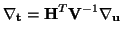 |
(3.24) |
and depends only on . The question of how sampling in the new coordinates is to be carried out is not well-addressed in the literature. Suppose, for example, that we wish to use embedding (3.22). Grid definition proceeds by letting
![$ {\bf t} = \Delta [n_{1}, n_{2}, n_{3}, n_{4}, n_{5}]^{T}$](img590.png) , where
, where  ,
are integers. Clearly, then, using (3.21a), grid points in the original coordinates are given by
,
are integers. Clearly, then, using (3.21a), grid points in the original coordinates are given by
![$ {\bf u} = [\Delta(n_{1}-n_{3}), \Delta (n_{2}-n_{4}), \frac{\Delta}{v_{0}}(n_{1}+n_{2}+n_{3}+n_{4}+n_{5})]^{T}$](img592.png) , and thus any point of the form
, and thus any point of the form
![$ {\bf u} = [\Delta m_{1}, \Delta m_{2}, \frac{\Delta}{v_{0}}m_{3}]^{T}$](img593.png) , for integer
, for integer  ,
,  and
and  is in the range of
 for some choice of the . This defines the rectilinear grid in the untransformed coordinates. Note, however, that not all of these points can be mapped back to some with
under (3.21b). This is worthy of note, but will not influence the numerical methods which will depend on discretizing directional derivatives in the coordinates, which, as mentioned above, are defined in terms of and not
for some choice of the . This defines the rectilinear grid in the untransformed coordinates. Note, however, that not all of these points can be mapped back to some with
under (3.21b). This is worthy of note, but will not influence the numerical methods which will depend on discretizing directional derivatives in the coordinates, which, as mentioned above, are defined in terms of and not
 .
We remark that the inverse relationship for (3.25) will be given by
.
We remark that the inverse relationship for (3.25) will be given by
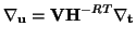 |
(3.25) |
where
 is the transpose of
.
is the transpose of
.
We don't wish to go too much into the formalism of these coordinate transformations here; it seems excessive since the associated circuit manipulations which we will review are quite straightforward. As mentioned earlier, the coordinate changes in this section are introduced in order to aid in understanding the method and MD-passivity, and are not necessary for deriving WDF-based algorithms for numerical integration, though it would appear that some types of reference circuits can only be derived via the transformation approach [130].
Next: MD-passivity
Up: Coordinate Changes in Higher
Previous: Coordinate Changes in Higher
Stefan Bilbao
2002-01-22