Next: MD Circuit Elements
Up: Multidimensional Wave Digital Filters
Previous: Embeddings
MD-passivity
In dealing with networks and circuit elements in multiple dimensions, we must have a means of generalizing their energetic properties accordingly. In particular, the notion of passivity, which in the lumped case played an important role in developing stable digital filters directly from an analog network, must be expanded to include the distributed character of the system to be modeled. The definition of MD-passivity was given in [48], and more basic results are provided in [85] and [131]. The idea is nearly the same as in the lumped case--a passive  -port cannot produce energy on its own, and hence a well-defined [12] network made up of Kirchoff connections of such passive -ports recirculates and possibly dissipates energy. The difference is that in MD, we would like to be able to take into account that for most physical systems, conservation of energy is a property holding with respect to time alone. We will need to make use of the coordinates defined in §3.3, so as to ensure that passivity holds with respect to all coordinates in the problem. In this section, we recap the main points of the definitions and derivations in [48].
Figure:
 -dimensional domain
  .
.
 |
We begin by defining a domain in the vector space defined by the new coordinates
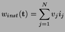
![$ {\bf t} = [t_{1},\hdots, t_{k}]^{T}$](img602.png) under a transformation of the type (3.21) (which may be an embedding). Consider an -port defined over the domain , with port voltages
under a transformation of the type (3.21) (which may be an embedding). Consider an -port defined over the domain , with port voltages
 and currents
 , for
, for
 . The instantaneous absorbed power density, at any point in the interior of is defined by
and the stored energy flow as a vector field
In addition, we can define the source and dissipated power densities within to be
 and
and
 . The energy balance of the -port can then be generalized directly from (2.3):
 |
(3.26) |
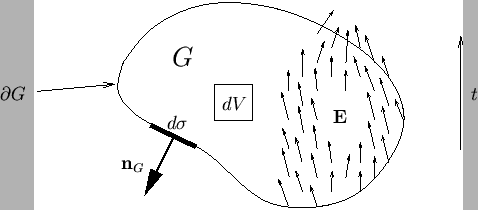
where
 is the -element row vector outward unit normal to the surface of ,
  is a surface element of , and
  is a volume element internal to . See Figure 3.3
 for a graphical representation of some of the relevant quantities. The -port is called MD-passive if there is a stored energy vector field
  , which is a positive semi-definite function of the state of the -port (i.e., all components of are non-negative, everywhere in ) such that
 |
(3.27) |
and MD-lossless if (3.28) holds with equality. The total stored energy lost through the boundary of must be less than the energy supplied through the ports in ; this is equivalent, from (3.27) to saying that the energy dissipated in must be greater than the energy coming from the source. The previous definition of MD-passivity has been more precisely called integral MD-passivity (with respect to a domain ) [85]. A corresponding differential (pointwise) definition is
  |
(3.28) |
An -port which is differentially MD-passive everywhere throughout a domain will also be integrally MD-passive with respect to . The converse is not necessarily true.
It is also useful to define, for an -port, a scalar total energy [85] by
 |
(3.29) |
Here  a spatial region defined as the cross-section of at time
  , and
, and
 is a column unit vector in the time direction; note that this definition is framed in terms of the untransformed coordinates
  , and has been projected onto these coordinates under (3.21a). It can also be used as a measure of the total energy at time in a given circuit, as we will see in §3.7.4.
Fettweis [44] looks at an extension of the idea of positive realness (see §2.2.2) to two dimensions, for the case of a real linear and shift-invariant -port. This idea generalizes easily to higher dimensions, as per some very early work in MD system theory [135]. Consider a real linear and shift-invariant (LSI) -dimensional -port, where the port quantities are in an exponential state of frequency
 , where
are the frequency variables conjugate to  . Thus we have the real instantaneous voltages and currents
where
 and
and
 are complex amplitudes.
If there is an impedance relation between the voltages and currents, then we can write
are complex amplitudes.
If there is an impedance relation between the voltages and currents, then we can write
where
![$ \hat{{\bf v}} = [\hat{v}_{1}, \hdots, \hat{v}_{N}]^{T}$](img626.png) and
and
![$ \hat{{\bf i}} = [\hat{i}_{1}, \hdots, \hat{i}_{N}]^{T}$](img627.png) .
The total complex MD power density at frequency
.
The total complex MD power density at frequency
 can be defined as
and the average or active power density as
The positive realness condition on  for MD-passivity follows immediately, and is similar to (2.5), except that we now must have
 for for |
(3.30) |
Thus the impedance must be positive real in all the new coordinates. The -port is MD-lossless if (3.31) holds with equality for Re ,
,
 . It is important to note that because of (3.26) and (3.25), we have
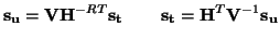 |
(3.31) |
where
![$ {\bf s}_{{\bf u}} = [s_{x_{1}},\hdots,s_{x_{n}},s_{t}]^{T}$](img636.png) is the vector of frequencies in the untransformed coordinates .
Thus, due to the positivity condition on the elements of the last row of
is the vector of frequencies in the untransformed coordinates .
Thus, due to the positivity condition on the elements of the last row of
 and the last column of
 , we will have that
 for for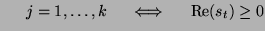 |
|
so that for an MD-passive -port,
 for for |
(3.32) |
It is thus seen that MD-passivity can be interpreted as passivity, but spread over a new system of coordinates (regardless of whether the new coordinates number more than the old).
Next: MD Circuit Elements
Up: Multidimensional Wave Digital Filters
Previous: Embeddings
Stefan Bilbao
2002-01-22