Next: Phase and Group Velocity
Up: Incorporating the DWN into
Previous: Higher-order Accuracy Revisited
Maxwell's Equations
We now take a brief look at Maxwell's equations, the (3+1)D system of PDEs which describes the time evolution of electromagnetic fields. This system was the original motivation behind the development of FDTD [184,214], and MDWD network methods for Maxwell's system were explored early on in [50]. In the interest of solidifying the link between these two types of methods, we show how a passive circuit representation yields a DWN, which is no more than a scattering form of FDTD.
Maxwell's Equations, for a linear isotropic (though not necessarily spatially homogeneous) medium, are usually written in vector form as
as
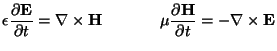 |
(4.127) |
where
![$ {\bf E} = [E_{x}, E_{y}, E_{z}]^{T}$](img2219.png) and
and
![$ {\bf H} = [H_{x}, H_{y}, H_{z}]^{T}$](img2220.png) are, respectively, the electric and magnetic field vectors,
are, respectively, the electric and magnetic field vectors,
 and
and
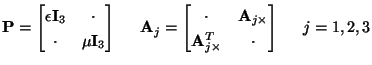
 are the dielectric constant and magnetic permeability of the medium, assumed positive and bounded away from 0. (We have left out losses here.) This system has the form of (3.1), with
![$ {\bf w} = [{\bf E}^{T}, {\bf H}^{T}]^{T}$](img2223.png) , and
, and
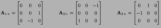
where
 is the
  identity matrix,
  stands for zero entries, and where we also have
Subsections
Next: Phase and Group Velocity
Up: Incorporating the DWN into
Previous: Higher-order Accuracy Revisited
Stefan Bilbao
2002-01-22