


Next: Embeddings
Up: Coordinate Changes and Grid
Previous: Coordinate Changes in (1+1)D
Coordinate Changes in Higher Dimensions
There are more choices for the type of coordinate transformation (and hence the type of grid) that are available when we move to higher dimensional problems. As an example, let us look at the transformation defined by:
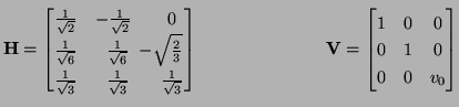 |
(3.19) |
which is discussed in [62] and [211].
Uniform sampling in the
 coordinates yields the grid arrangement shown in Figure 3.2(a), flattened onto the
  plane. This is, effectively, a cubic lattice of points viewed along its main diagonal.
Figure 3.2:
(2+1)D sampling grids, (a) in hexagonal and (b) rectangular coordinates.
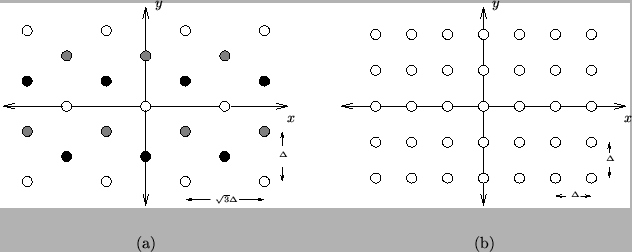 |
At any given time step, one of three different grids (in Figure 3.2(a) the different grids are marked by grey, white or black points) which are simple translations of each other, is used. In a discrete setting, it is sometimes possible (depending on the system at hand) to design an algorithm such that they are used cyclically--grid variables at white grid points can be updated with reference to variables at the grey points, which in turn were updated using stored variables at the black points, etc. If the separation of the points is as indicated in Figure 3.2(a), then we have used sample steps of
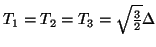 .
.
Subsections
Next: Embeddings
Up: Coordinate Changes and Grid
Previous: Coordinate Changes in (1+1)D
Stefan Bilbao
2002-01-22