Coordinate Changes in (1+1)D

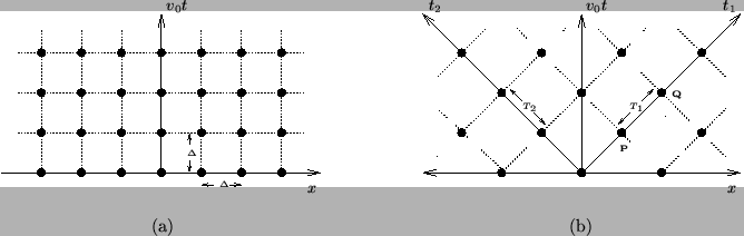
Solving a set of PDEs numerically nearly always involves sampling the problem domain, and attempting to approximate the solution to the problem at the finite collection of points. Coordinate sampling in the MDWDF context was first examined in [122], and was subsequently addressed in [62] and [7]. In (1+1)D, there is essentially only one useful type of regular grid; it is shown, in the (1+1)D case, in Figure 3.1(a), where the grid spacings or step sizes are assumed equal to $\Delta$ in the scaled time (i.e., $t' = v_{0}t$) and space directions. Note that the use of the scaled coordinates allows this uniform sampling, without implying any restriction on the relative grid spacings in the unstretched coordinates, since we have introduced the (as yet) free parameter $v_{0}$.

Figure 3.1: Sampling grids, (a) in rectangular coordinates $(x,v_{0}t)$ and (b) in the new coordinates $(t_{1}, t_{2})$ defined by (3.18).

Suppose we now change coordinates by:

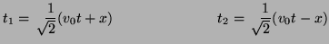$$t_{1} = \hspace{0.1in}\frac{1}{\!\!\!\!\sqrt{2}}(v_{0}t+x)\hspace{1.0in}t_{2} = \hspace{0.1in}\frac{1}{\!\!\!\!\sqrt{2}}(v_{0}t-x)$$ (3.17)

which corresponds to a transformation of type (3.15) with

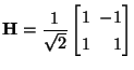$$\mathbf{H} = \frac{1}{\sqrt{2}}\begin{bmatrix}1&\!\!\!-1\\ 1&\,\,1\\ \end{bmatrix}$$ (3.18)

If we now sample the plane in the $(t_{1}, t_{2})$ coordinates, with equal spacings along the two axes, using a step size of $T_{1}=T_{2}$, we obtain the grid in Figure 3.1(b). Notice that if we choose 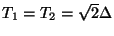$T_{1}=T_{2}=\sqrt{2}\Delta$, then our grid aligns perfectly with exactly half of the grid points sampled uniformly along the $(x,v_{0}t)$ axes, as in Figure 3.1(a). In fact, the grid of Figure 3.1(a) can be decomposed into two grids of the form in Figure 3.1(b), where one of the grids is shifted by $(\Delta,\Delta)$ with respect to the other, in the $(x,v_{0}t)$ plane. It will be possible in some instances to exploit this decomposition so as to achieve a gain in computational efficiency; the key idea here is that if we begin with a grid such as shown in Figure 3.1(a), and then are able to develop an algorithm such that only one of the two subdomains is used, then we will have halved the amount of computation, at the expense of a decrease in accuracy by a factor of $\sqrt{2}$ (the step size in the $(t_{1}, t_{2})$ plane is $T_{1}=T_{2}=\sqrt{2}\Delta$ versus $\Delta$ in the $(x,v_{0}t)$ plane). We will mention this offset sampling [61,211] when we look at the (1+1)D transmission line problem in §3.7, and will examine subgrid decompositions extensively in §4.4.3 and Appendix A. It is important to point out that regardless of the coordinate change, updating in any of the WDF-based algorithms that will subsequently be developed will be done with respect to the time variable alone (the direction of data flow is still in the time direction), as per standard explicit finite difference methods for hyperbolic problems.