The (1+1)D Transmission Line

As a slightly more involved example, which highlights some of the issues which typically arise in the construction of these algorithms, consider the (1+1)D transmission line or telegrapher's equations [63]:

$$\begin{eqnarray}l\frac{\partial i}{\partial t}+\frac{\partial u}{... ...c{\partial u}{\partial t}+\frac{\partial i}{\partial x}+gu+h&=&0 \end{eqnarray}$$ (3.52a)

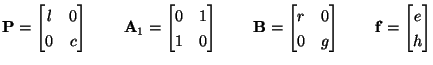
Here, $i(x,t)$ and $u(x,t)$ are the current and voltage in the transmission line, $l$, $c$, $r$ and $g$ are inductance, capacitance, resistance and shunt conductance per unit length respectively, and are all non-negative functions of $x$ ($l$ and $c$ are strictly positive). $e(x,t)$ and $h(x,t)$ represent distributed voltage and current source terms. System (3.56) is symmetric hyperbolic; it has the form of (3.1), with ${\bf w} = [i,u]^{T}$, and

$${\bf P} = \begin{bmatrix}l&0\\ 0&c\\ \end{bmatrix}\hspace{0.3in}{... ...0&g\\ \end{bmatrix}\hspace{0.3in}{\bf f} = \begin{bmatrix}e\\ h\\ \end{bmatrix}$$ (3.53)