MDKC for the (1+1)D Transmission Line Equations

In order to put this system into the form of an MDKC, let us first change dependent variables by

$$i_{1} \triangleq i\hspace{1.0in}i_{2} \triangleq \frac{u}{r_{0}}$$ (3.56)

where $r_{0}>0$ is a free constant parameter which has dimensions of resistance. The primary reason for introducing this parameter is so that the numerical algorithm may later be tuned to be optimally efficient (in terms of the largest allowable time step for a given grid spacing). After changing variables, and multiplying the second equation by $r_{0}$, we obtain:

$$\begin{eqnarray}l\frac{\partial i_{1}}{\partial t}+r_{0}\frac{\pa... ..._{0}\frac{\partial i_{1}}{\partial x}+gr_{0}^{2}i_{2}+r_{0}h&=&0 \end{eqnarray}$$ (3.57a)

At this point, it is already possible to write the above system in the form of an MDKC, which is shown in Figure 3.11(a).

Figure 3.11: MDKCs for the (1+1)D transmission line system (3.61)-- (a) a direct representation, and (b) after splitting and shifting inductances.

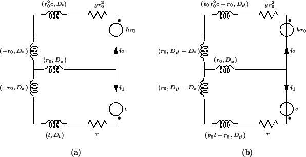
Kirchoff's node equation tells us the current in the common branch, which is $i_{1}+i_{2}$, then the loop conditions yield system (3.61). This representation, however, can not give an explicit algorithm, because of the purely spatial MD inductors which form a T-junction between the two loops; that is, if one tries to treat these as one-ports, their WD counterparts will be found to contain delay-free paths from input to output; in other words, the algorithm will be implicit. Nor can it be considered to be MD-passive, since there are negative inductances. By performing a few network theoretic transformations to this MDKC, we can obtain a representation which is MD-passive, and which will give rise to an explicit numerical method. The idea here, grossly speaking, is to make sure that each inductance is positive, and that every inductor ``points'' in the direction of a transformed coordinate, as per conditions (3.14).

First note that we can split and shift the differential operators around at will, as long as the loop equations remain unchanged. In particular, we can redraw the circuit as in Figure 3.11(b), where we have introduced the scaled time coordinate $t' = v_{0}t$ and its associated derivative $D_{t'}$. Now, examine the three inductors which form a T-junction connecting the two loops. If we are planning to use coordinates defined by (3.19), then the two inductors on the vertical rail can be identified as MD-passive--we have $D_{t'}-D_{x} = \sqrt{2}D_{2}$. The inductance in the common branch, however is not yet in proper form. It is now possible to apply transformations from classical network theory so as to ensure that the resulting equivalent two-port is composed of only MD-passive elements. Although the system as a whole does not change under these manipulations, we would like it to be concretely passive, so that it may be decomposed into a connection of simpler passive blocks. Since the two-port containing the T-junction will always be, by itself, linear and shift-invariant (i.e., shift-invariant with respect to any coordinate, because the inductances are constant), we are justified in describing it by means of impedances and applying spectral transformations. When it is connected to the other components which are not shift-invariant, the spectrally transformed two-port may be interpreted in terms of differencing formulae.

Figure 3.12: Equivalent two-ports-- (a) T-junction, with impedances $Z_{A}$ and $Z_{B}$ and (b) and (c), lattice and Jaumann equivalent two-ports, both with $Z_{1} = Z_{A}$ and $Z_{2} =Z_{A}+2Z_{B}$.

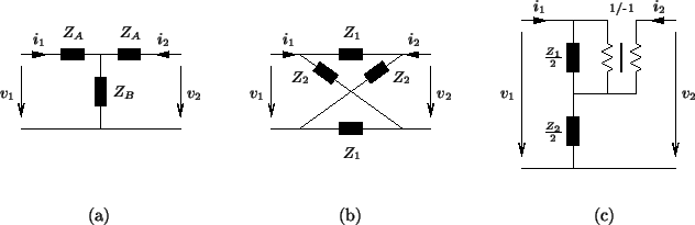The symmetric T-junction, and its lattice [55,131] and Jaumann [132] equivalents are shown in Figure 3.12, for arbitrary impedances $Z_{A}$ and $Z_{B}$. Replacement of the T-junction in Figure 3.11(b) by either of the two-ports in Figure 3.12(b) and (c) gives an MDKC which is indeed concretely MD-passive; this circuit is shown in Figure 3.14(a). Note that in this representation, we have left inductors (with symbols $D_{t'}$) in the circuit, instead of rewriting them as $D_{t'} = (D_{1}+D_{2})/\sqrt{2}$. In this case, we must proceed as such because their inductances are possibly spatially-varying (note that they depend on $l$ and $c$); for this reason these elements cannot be split into inductances acting along directions $t_{1}$ and $t_{2}$ without giving up passivity. For these inductances, we will apply the generalized trapezoid rule, which was discussed in §3.5.1.