Next: A MDWD Network for
Up: The (1+1)D Transmission Line
Previous: MDKC for the (1+1)D
Digression: Derivation of an Inductive Lattice Two-port
We have derived the WD equivalents for all the standard circuit elements, but the two-ports pictured in Figure 3.12 need a special treatment. Fettweis and Nitsche find the lattice form to be the most straightforward derivation, but we would especially like to call attention to the fact that the resultant WD two-port is the same regardless of which of the equivalent structures we choose; use of a concretely MD-passive two-port, however, makes the passivity of the resulting circuit obvious. We will continue to use the Jaumann equivalent in all future diagrams (though we could equally well use the lattice form). Basu [10], as well as Fettweis [46] make the point that an electrical network equivalent is a convenient formalism for developing MD-passive discrete networks, but it is by no means necessary.
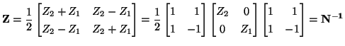
Beginning from any of the equivalent two-port structures in Figure 3.12, we can immediately write down the impedance matrix, which we will denote by
 :
:
where we have set
![$ \mathbf{N}=\bigl[\begin{smallmatrix}
1&\,\,1\\
1&\!\!-1\\
\end{smallmatrix}\bigr]$](img800.png) and
and  =
=
![$ \bigl[\begin{smallmatrix}
Z_{2}&0\\
0&Z_{1}\\
\end{smallmatrix}\bigr]$](img802.png) .
.
We now introduce a port resistance matrix
![$ \mathbf{R}=\bigl[\begin{smallmatrix}
R&0\\
0&R\\
\end{smallmatrix}\bigr]>{\bf0}$](img803.png) , where we can choose equal port resistances because the two-port is symmetric. The scattering matrix is then, from (2.21),
, where we can choose equal port resistances because the two-port is symmetric. The scattering matrix is then, from (2.21),
where
 is the
  identity matrix. This is easily rearranged to become
Returning to the problem of the (1+1)D transmission line, for the two-port in question in Figure 3.14(a), we have
 and
and
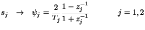
 . Notice in particular that for these choices of impedance, any of the two-ports of Figure 3.12 are described by MD positive real matrices. We now discretize using the trapezoid rule, i.e.
where we also will set
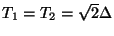 . If we make the choice
 , we obtain the discrete-time, causal scattering matrix
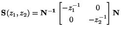 |
(3.58) |
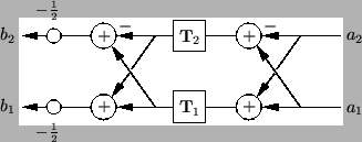
The resulting MD two-port is shown in Figure 3.13.
Figure 3.13:
Signal flow diagram for the MDWD lattice or Jaumann two-port.
 |
It should be clear that the same procedure can be used for arbitrary impedances  and
and  ; it should be remarked, however, that we can not always get a simple form without a through path like that pictured in Figure 3.13. Since this two-port is strictly causal, it may easily be connected to other ports without the risk of the appearance of a delay-free loop.
Next: A MDWD Network for
Up: The (1+1)D Transmission Line
Previous: MDKC for the (1+1)D
Stefan Bilbao
2002-01-22