Next: Other MD Elements
Up: MD Circuit Elements
Previous: MD Circuit Elements
The MD Inductor
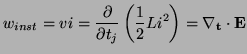
Consider the following (partial) differential equation:
 |
(3.33) |
where  is a positive constant, and
  , for any
  ,
,
 is a coordinate defined by transformation (3.21). We now have
 and
and
 . Considered as an MD one-port, the instantaneous applied power will be
if we also define the stored energy flux  to be
to be
 |
(3.34) |
where
 is a column unit vector in the direction. If
  , this is indeed a positive semi-definite vector function of the current across the one port. (3.34) defines a passive (in fact lossless) element in the sense of (3.29), henceforth called an MD-inductor, of inductance and direction .
This equation resembles that which defines the voltage/current relation in an inductor with inductance , the exception being that the integration variable is no longer time, but , a mixed space-time variable. In fact, the discretization procedure is identical to that of the lumped case, as we shall see, but for illustrative purposes, we will derive the multidimensional wave digital one-port. The important thing to note here is that even though (3.34) is defined over a  -dimensional domain with coordinates
  , it is solved (given
  , say) as a series of one-dimensional integrations (since (3.34) must hold for all values of t).
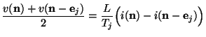
We can immediately approximate (3.34) by the MD trapezoid rule [62] as
 |
(3.35) |
where
 .
.  is interpreted as the step-size.
Assuming that we have uniformly sampled the plane as in §3.3, with grid spacings
is interpreted as the step-size.
Assuming that we have uniformly sampled the plane as in §3.3, with grid spacings
 , we now define the grid functions
 and
and
 where
where
![$ {\bf n} = [n_{1},\hdots, n_{k}]^{T}$](img657.png) is an integer-valued vector. We intend to use them to approximate
is an integer-valued vector. We intend to use them to approximate
![$ v({\bf t}=[n_{1}T_{1},\hdots,n_{k}T_{k}]^{T})$](img658.png) and
and
![$ i({\bf t}=[n_{1}T_{1},\hdots n_{k}T_{k}]^{T})$](img659.png) , so we can immediately write the recursion
, so we can immediately write the recursion
 |
(3.36) |
which approximates (3.34) to
 .
.
We can now introduce the wave variables,
which are also grid functions defined over  . As in the lumped case,
  is an arbitrary positive number (here assumed constant). Inserting these wave variables into (3.37) yields, with the choice
 ,
,
 |
(3.37) |
In terms of the untransformed coordinates (where we will perform the updating in a simulation), (3.36) becomes
 |
(3.38) |
again to second order in the transformed spacing. The quantity
 is the vector corresponding to the same shift, in the untransformed coordinates.
Take, for example the case of an inductor of direction  under the coordinate change defined by (3.19). A shift of
 of
of  in direction corresponds to a shift in the old coordinates of
![$ (T_{1}/\sqrt{2})[1, 1/v_{0}]^{T}$](img673.png) . Referring to Figure 3.1(b), where we have chosen
. Referring to Figure 3.1(b), where we have chosen
 , the instance of the wave variable
  entering the MD-inductor at point
  exits, sign-inverted, as
  at point
  . From this standpoint, MD-losslessness is obvious, since the MD-inductor merely shifts and sign-inverts an array of numbers.
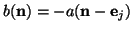
One point requires some clarification; the MD inductor as defined by (3.34) is MD-passive for constant , and for a transformed coordinate ,
. In problems for which material parameters have some spatial variation, some of the MD circuit elements that we will require will, as a rule, have some spatial dependence. If in (3.34) is a function of , then in general the equation does not describe an MD-passive one-port. More precisely, if does not commute with
 , then the application of the trapezoid rule to (3.34) does not yield the simple wave relationship (3.38). This begs the question, then, of how the trapezoid rule can be applied to circuit elements which are not LSI (which we will require in order to numerically integrate systems with spatial material parameter variation).
For almost all the systems of interest in this thesis, it will be possible to consolidate any material parameter variation in circuit elements defined with respect to the pure time direction (recall that in our general symmetric hyperbolic system (3.1), such variation is confined to the coefficients of the time derivative term). For example, consider an inductor described by
 |
(3.39) |
in the (1+1)D coordinates defined by (3.18). Here, is strictly positive, but may be a function of  , and note that
  is not among the new coordinates defined by (3.18). Because does commute with
 , it is still possible to apply the trapezoid rule, in the time direction, in order to get a wave relationship of the form of (3.38). The directional shift will then be along the time direction, and we need to be sure that the shift does in fact refer to another grid point--from Figure 3.1(b), we can see that this is in fact true (it is true for any of the coordinate systems discussed in §3.3). It is of course possible to include a pure time derivative among the new coordinates; this is done, for example, in the case of the embedding defined by coordinates (3.22), for which
  is simply
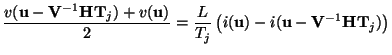
  multiplied by a scaling factor. Nitsche [62] has called this the generalized trapezoid rule. Note, however, that if we write (3.40) as
 |
(3.40) |
it is not permissible to treat this as a series connection of two MD inductors--neither one is MD-passive, because does not commute with either of the two directional derivatives.
A more general definition of an inductor, suitable for use in time-varying or nonlinear problems is
 |
(3.41) |
for any transformed coordinate . In this case, can depend on or even on or  ; as long as we have and use power-normalized waves, the MD inductor defined by (3.42) is MD passive [48,85]. For constant , (3.42) reduces to (3.34). Circuit elements of this type appear in circuit networks for fluid dynamical systems [16,49,70,191], as well as in a vector-matrix context when dealing with the linearized Euler Equations [86]. We also note that passivity under time-varying conditions can be enforced as it has been done in digital waveguide networks [166]; it would appear that waveguide networks (to be discussed in depth in Chapter 4) could be generalized to include the nonlinear case in the same manner (see Appendix B for an interesting application of these ideas).
Next: Other MD Elements
Up: MD Circuit Elements
Previous: MD Circuit Elements
Stefan Bilbao
2002-01-22