An Upwind Form

One of the interesting (and only briefly mentioned [86]) features of the MDKC representation is that it can easily be manipulated to yield what are known as upwind difference methods; such methods are usually applied to problems for which there is a directional bias in the propagation speed, and are heavily used in fluid dynamical calculations [89].

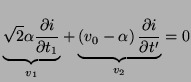
We can rewrite the advection equation (3.51), where we assume, without loss of generality, that $\alpha > 0$ as

$$\underbrace{\sqrt{2}\alpha\frac{\partial i}{\partial t_{1}}}_{v_{... ...underbrace{\left(v_{0}-\alpha\right)\frac{\partial i}{\partial t'}}_{v_{2}} = 0$$

which can be written as the MDKC shown in Figure 3.9(a). We now have

$$L_{1} = \sqrt{2}\alpha \hspace{1.0in}L_{2} = v_{0}-\alpha$$

Figure 3.9: An upwind-differencing form for the advection equation-- (a) MDKC and (b) MDWD-network.

In this case, we have left a directional derivative in the pure time (or scaled time) direction in the MDKC; for this inductor, we apply the generalized trapezoid rule discussed in §3.5.1, with a step-size of $T' = \Delta$. The resulting MDWD network is shown in Figure 3.9(b), with port resistances given by

$$R_{1} = \frac{2\alpha}{\Delta}\hspace{1.0in}R_{2} = \frac{2}{\Delta}\left(v_{0}-\alpha\right)$$ (3.51)

(Note that a directional shift of length $\Delta$ in the scaled time direction $t' = v_{0}t$ corresponds to a pure time shift of duration $\Delta/v_{0} = T$, and so we have indicated this shift in Figure 3.9(b) by a ${\bf T}$). The signal flow graph, with spatial dependence expanded out, is shown in Figure 3.10.

Figure: Signal flow graph for Figure 3.9(b), for $\alpha > 0$.

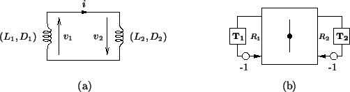
This structure is in a sense, a better model for the advection system; recall that for $\alpha > 0$, the solution at any future time instant $t\geq 0$ will simply be the initial distribution shifted to the right by an amount $\alpha t$. By using upwind differencing, we have dispensed with the unphysical leftward traveling wave which appears in the signal flow diagram in Figure 3.7. As before, the network will be MD-passive for $v_{0}\geq \alpha$. It also degenerates to a simple delay line when $v_{0}=\alpha$ (in which case we will have $R_{2} = 0$, and the right-hand inductor in Figure 3.9(b) can be dropped from the network).

Because all the systems that we will subsequently examine do not have any directional disparities in the wave speed, we will not pursue the subject of upwind differencing further here. We do mention, though, that digital waveguide networks [166,198], which are intimately related to MDWD networks, are incapable of performing upwind differencing for the simple reason that they are constructed from bidirectional delay lines (or unit elements), which carry information symmetrically in opposite directions. In this respect, the two approaches stand in stark contrast; the advantage of having an MD representation is very clear in this case.