Simplified Networks

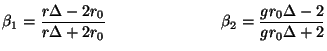
In the particular case for which $l$ and $c$ are constants, and where we do not have sources, the MDWD network shown in Figure 3.14(b) can be simplified considerably. If we pick $v_{0}=1/\sqrt{lc}$ and $r_{0} = \sqrt{l/c}$, then $R_{1}$ and $R_{2}$ become zero, and their associated inductors may be dropped from the network (that is, they can be treated as short-circuits). The two series adaptors then reduce to simple multiplies of the signals output by the lattice two-port as in Figure 3.15(a) where we have written

$$\beta_{1} = \frac{r\Delta-2r_{0}}{r\Delta+2r_{0}}\hspace{1.0in}\beta_{2} = \frac{gr_{0}\Delta-2}{gr_{0}\Delta+2}$$

Figure 3.15: Simplified MDWD network for the (1+1)D transmission line equations-- (a) for constant $l$ and $c$ and (b) further simplified in the distortionless case.

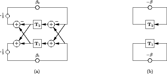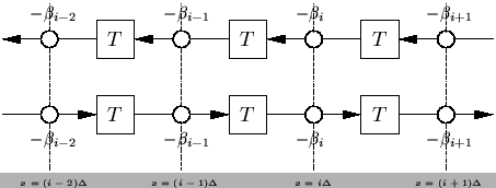
If, in addition, the transmission line is distortionless [28], so that we have $lg = cr$ for all values of $x$ (though as mentioned above, we require $l$ and $c$ to be constant), then the network can be simplified further giving Figure 3.15(b), where $\beta_{1}=\beta_{2}=\beta$. Now the MDWD network has decoupled into two independent loops, each comprised of an MD shift and a scaling. Examine the expanded signal flow graph of Figure 3.16, where the value of the multiplier coefficient $-\beta$ at location $x=i\Delta$ is written as $\beta_{i}$. Values input into the upper array will be shifted repeatedly to the left and attenuated by the factor $-\beta$, and similarly, those in the lower array are shifted to the right and attenuated by the same factor. We thus have a traveling wave formulation of the solution to the transmission line equations, to be compared with the digital waveguide implementation to be discussed in Chapter 4.

Figure 3.16: Signal flow graph for the MDWD network of Figure 3.15(b).

Two special cases are of note here. If the transmission line is lossless, so that $r=g=0$, then $\beta = -1$. The initial values in the storage registers are shifted without attenuation. We would like to note, however, that if $\Delta>\frac{2}{gr_{0}}$, then $\beta>0$, and the traveling waves will be oscillatory, and the solution is thus non-physical. More disturbing is the case $\Delta=\frac{2}{gr_{0}}$, in which case we have $\beta = 0$, and all energy leaves the network immediately! Though these examples would seem to indicate that the MDWD network is not behaving correctly, it should be kept in mind that, by construction, it is stable and consistent with the continuous time/space transmission line equations, and is convergent in the limit as $\Delta\rightarrow 0$, by the Lax-Richtmeyer Equivalence Theorem [176]. $\Delta$ can always be chosen small enough so that $\beta$ is negative, and that thus the solution will be well-behaved (i.e., non-oscillatory). This important extra restriction on the grid spacing, which is independent of the time step, is purely a result of the use of the trapezoid rule as our integration method. The lesson here is that passivity, while providing a guarantee of stable numerical methods, does not ensure that we necessarily get a physically acceptable solution in all cases.