


Next: Coordinate Changes in (1+1)D
Up: Coordinate Changes and Grid
Previous: Coordinate Changes and Grid
These same authors provide some more detailed guidelines as to what types of coordinate changes are of interest [62]. In particular, they describe transformations of the form:
 |
(3.14a) |
where
![$ \mathbf{t} = [t_{1},\hdots, t_{n+1}]^{T}$](img538.png) are the new coordinates and
are the new coordinates and
![$ \mathbf{u}=[x_{1},\hdots,x_{n},t]^{T}$](img539.png) are the old.
are the old.
 is prescribed to be diag
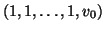 and can be thought of as a simple scaling of the original coordinates
  to a non-dimensional (or rather, ``all-spatial'') form.
  thus plays an important role, as we shall see later in a discrete setting, as the space step/time step ratio on a numerical grid. Its magnitude will be governed by a stability bound [176], sometimes called the Courant-Friedrichs-Lewy (CFL) criterion, as in conventional explicit finite difference methods (although the manifestation of the condition in the networks we will derive is of a quite different character). The invertible matrix
 is usually chosen to be orthogonal [62].
Here, we can see that the requirement (3.14a) will be satisfied if the elements in the rightmost column of
 are positive; if
  is orthogonal, we have
 . The bottom row of then consists of positive elements (often chosen equal, so as to give equal contributions from all components
  to
to  ), in order to satisfy requirement (3.14b).
The differential operators
![$ \nabla_{\mathbf{t}}=[\frac{\partial}{\partial t_{1}}, \hdots ,\frac{\partial}{\partial t_{k}}]^{T}$](img549.png) and
and
![$ \nabla_{\mathbf{u}}=[\frac{\partial}{\partial x_{1}}, \hdots ,\frac{\partial}{\partial x_{n}},\frac{\partial}{\partial t}]^{T}$](img550.png) are related by:
are related by:
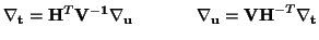 |
(3.15) |
Also, we introduce the scaled time variable
 |
(3.16) |
which will necessitate a special treatment in the circuit models to follow. See §3.5.1 for more details.
Next: Coordinate Changes in (1+1)D
Up: Coordinate Changes and Grid
Previous: Coordinate Changes and Grid
Stefan Bilbao
2002-01-22