Incorporating Losses and Sources

We now reconsider the full (1+1)D transmission line equations, including the effects of losses and sources; this system was presented earlier in §3.7, and we repeat its definition here:

$$\begin{eqnarray}l\frac{\partial i}{\partial t}+\frac{\partial u}{... ...c{\partial u}{\partial t}+\frac{\partial i}{\partial x}+gu+h&=&0 \end{eqnarray}$$ (4.54a)

Here $r(x)\geq 0$ and $g(x)\geq 0$ represent resistance and shunt conductivity at any point in the domain, and $e$ and $h$ are driving terms and can be functions of $x$ and $t$.

In order to add these terms to the centered difference approximation in such a way that we may still use an interleaved scheme, we can use the semi-implicit [184] approximations to $i$, and $u$ given by

$$i(x,t) = \frac{1}{2}\left(i(x,t-T/2)+i(x,t+T/2)\right) +O(T^{2})$$

$$u(x,t) = \frac{1}{2}\left(u(x,t-T/2)+u(x,t+T/2)\right) +O(T^{2})$$

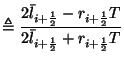
We also define

$$r_{i+\frac{1}{2}} \triangleq r\left((i+{\textstyle \frac{1}{2}})\Delta\right) g_{i} \triangleq g(i\Delta)\notag$$

$$e_{i+\frac{1}{2}}(n+{\textstyle \frac{1}{2}}) \triangleq e\left((i+{\textstyle \frac{1}{2}})\Delta,(n+{\textstyle \frac{1}{2}})T\right) h_{i}(n) \triangleq h(i\Delta,nT)\notag$$

and use the second-order approximations

$$\bar{e}_{i+\frac{1}{2}}(n) = \frac{1}{2}\left(e_{i+\frac{1}{2}}(n+{\textstyle \frac{1}{2}})+ e_{i+\frac{1}{2}}(n-{\textstyle \frac{1}{2}})\right)$$

$$\bar{h}_{i}(n-{\textstyle \frac{1}{2}}) = \frac{1}{2}\left(h_{i}(n)+h_{i}(n-1)\right)$$

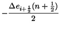
We then get, as an approximation to (4.43),

$$\begin{eqnarray}\hspace{-0.7in}I_{i+\frac{1}{2}}(n+{\textstyle \f... ...)+ \Delta\sigma_{U,i}\bar{h}_{i}(n-{\textstyle \frac{1}{2}}) = 0 \end{eqnarray}$$

with

$$\rho_{I,i+\frac{1}{2}} \triangleq \frac{2\bar{l}_{i+\frac{1}{2}}-r_{i+\frac{1}{2}}T}{2\bar{l}_{i+\frac{1}{2}}+r_{i+\frac{1}{2}}T} \rho_{U,i} \triangleq \frac{2\bar{c}_{i}-g_{i}T}{2\bar{c}_{i}+g_{i}T}$$

$$\sigma_{I,i+\frac{1}{2}} \triangleq \frac{2}{2v_{0}\bar{l}_{i+\frac{1}{2}}+r_{i+\frac{1}{2}}\Delta} \sigma_{U,i} \triangleq \frac{2}{2v_{0}\bar{c}_{i}+g_{i}\Delta}$$

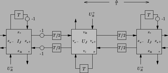
Losses and sources can be added to the waveguide network scheme rather easily, by introducing new ports at each series or parallel junction. In fact, as per wave digital filters, each pair of terms $ri+e$, and $gu+h$ can be interpreted as a resistive source [46], and only requires the addition of a single new port at each junction. (The resistive voltage source was discussed in §2.3.4.) For any parallel port we will call the new port admittance $Y_{R,i}$, and the voltage wave variable entering the port $U_{R,i}^{+}$. For a series port, we call the new impedance $Z_{R,i+\frac{1}{2}}$, and the incoming voltage wave variable $U_{R,i+\frac{1}{2}}^{+}$. The generalized network is shown in Figure 4.15, with the new loss/source port immittances marked.

Figure: Waveguide network for system (4.43).

As a result of the addition of this port, the junction admittances and impedances become

$$Y_{J,i} \triangleq Y_{x^{-},i}+Y_{x^{+},i}+Y_{c,i}+Y_{R,i}\hspace{0.5in}$$

$$Z_{J,i+\frac{1}{2}} \triangleq Z_{x^{+},i+\frac{1}{2}}+Z_{x^{-},i+\frac{1}{2}}+Z_{c,i+\frac{1}{2}}+Z_{R,i+\frac{1}{2}}\hspace{0.5in}$$

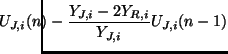
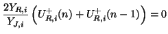
Beginning again from a parallel junction, and proceeding through a derivation similar to that which leads to (4.32), we obtain a difference relation among the junction voltages and currents:

$$\hspace{-0.4in}U_{J,i}(n) - \frac{Y_{J,i}-2Y_{R,i}}{Y_{J,i}}U_{J,i}(n-1) + \frac{2}{Y_{J,i}}\left(I_{J,i+\frac{1}{2}}(n-{\textstyle \frac{1}{2}})-I_{J,i-\frac{1}{2}}(n-{\textstyle \frac{1}{2}})\right)\notag$$

$$- \frac{2Y_{R,i}}{Y_{J,i}}\left(U_{R,i}^{+}(n)+U_{R,i}^{+}(n-1)\right)=0$$

In order to equate this relation with (4.44b), we can set

$$Y_{R,i} = g_{i}\Delta$$

$$U_{R,i}^{+}(n) = -\frac{h_{i}(n)}{2g_{i}}$$

Beginning from a series junction, we obtain an analogous relation, which becomes (4.44a) under the choices

$$Z_{R,i+\frac{1}{2}} = r_{i+\frac{1}{2}}\Delta$$

$$U_{R,i+\frac{1}{2}}^{+}(n+{\textstyle \frac{1}{2}}) = -\frac{\Delta e_{i+\frac{1}{2}}(n+{\textstyle \frac{1}{2}})}{2}$$

Note that in the case where the loss parameter $g$ is zero, or close to zero, $U_{R,i}^{+}(n)$ will become infinite, or very large. For this reason, it will be necessary in this case to use the dual type of wave; i.e., if $g_{i}$ is small, set $I_{R,i}^{+} = Y_{R,i}U_{R,i}^{+} = -\frac{\Delta}{2}h_{i}$, and use current waves at the series junctions. The other impedances in the network remain unchanged under the addition of losses and sources; thus all the stability criteria mentioned in §4.3.6 remain the same. It is rather interesting to note, however, that in the case of the current-centered network, for example (type II), scattering at the series junctions is no longer trivial if we have non-zero sources $e$ or loss $r$. That is, the series junctions cannot be treated as simple throughs. A similar statement holds for the dual case of the voltage-centered network (type I) in (1+1)D, but will not be true when we generalize to the (2+1)D mesh (see §4.4).