


Next: Boundary Conditions
Up: The (1+1)D Transmission Line
Previous: Incorporating Losses and Sources
Numerical Phase Velocity and Dispersion
We now make a few comments regarding the spectral properties of these difference methods; a detailed summary of spectral methods is provided in Appendix A.
Consider again the type II DWN for the (1+1)D transmission line equations, as discussed in §4.3.6. In the lossless, source-free case, the difference scheme can be written purely in terms of the junction voltages, and for integer time steps  as
as
 |
(4.56) |
where
 and
and
 , and the self-loop admittance is given by (4.38). In effect, we are numerically solving the reduced form (4.39) of (4.17) obtained by elimination of the current
  .
.
If the material parameters are constant, then (4.45) can be rewritten as
where
 and
and
 is the wave speed.
It is possible to examine this scheme in terms of discrete spatial frequencies
is the wave speed.
It is possible to examine this scheme in terms of discrete spatial frequencies  , as per the methods discussed in [176]; the range of spatial frequencies which are available on this grid of spacing
  are
are
 .
The spectral amplification factors (defined in §A.1) for this scheme are given by
.
The spectral amplification factors (defined in §A.1) for this scheme are given by
where
These spectral amplification factors define the numerical phase velocities
 [176] (see §A.1.4) and thus the numerical dispersion of the scheme (in general, the numerical phase velocity is different from the physical velocity
  ). It is of interest to plot the numerical phase velocity of this scheme versus that of the MDWDF for the same system; the spatial frequency dependence of the various modal frequencies of the MDWDF were discussed in §3.9.2.
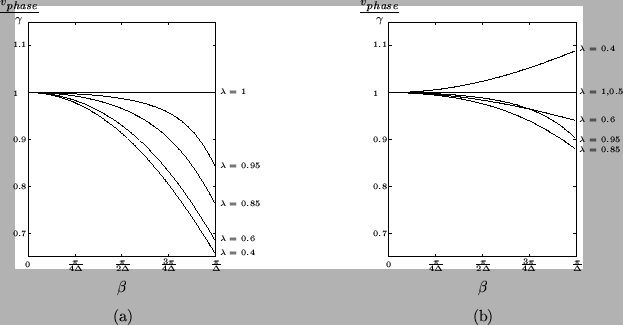
In Figure 4.16, the quantity
 is plotted for various values of the parameter
  . At the stability bound, for
 (i.e.
(i.e.
 ), both schemes are dispersionless. For the DWN, all spatial frequencies are slowed increasingly as is decreased, but for the MDWD network, wave speeds decrease for
 , then are exact again at
 , and finally faster than the physical speed if
 . This curious behavior of the phase velocities in the MDWD network was also mentioned in §3.9.2. In general, the phase velocities of the MDWD network are closer to the correct wave speed over the entire spatial frequency spectrum for a wide range of --this is mitigated, however, by the fact this MDWD network corresponds to a three-step difference method (compared to two-step for the DWN), and is thus more computationally intensive.
Figure:
Numerical dispersion curves for various values of -- (a) for the DWN and (b) for the MDWD network.
 |
Next: Boundary Conditions
Up: The (1+1)D Transmission Line
Previous: Incorporating Losses and Sources
Stefan Bilbao
2002-01-22