Boundary Conditions

The (1+1)D transmission line equations, if they are to be solved on a domain of finite extent, require one supplementary boundary condition at any end point [82]. Suppose that $x=0$ is such an end point, and furthermore assume that our grid has been constructed such that the point $x=0$ coincides with one of the parallel (grey) scattering junctions of the interleaved waveguide network shown in Figure 4.15. We now are faced with terminating the waveguide network, by replacing the left-hand port of the parallel junction at $x=0$ with a lumped network. If the lumped network is passive (that is, if its reflectance is bounded), then it should be clear that the network as a whole will be passive as well.

The two most important types of boundary condition are

$$u(0,t) =0 \mbox{{\rm Short-circuit at $x=0$}}$$

$$i(0,t) =0 \mbox{{\rm Open-circuit at $x=0$}}$$

Both are lossless, and have the form of (3.8). The first of these conditions is easy to deal with by short-circuiting the left-hand port. In this case, we may also remove the self-loop, as well as the combined loss/source port from the junction at $x=0$. $U_{J,0}$ is forced to zero by the short-circuit condition; this boundary termination is shown in Figure 4.17(a). We have assumed that $Y_{x^{+},0} = Y_{x^{-},0}$, so that the termination degenerates to a simple sign inversion of the wave incoming from the right-hand side.

Figure 4.17: Boundary terminations of the waveguide network for the (1+1)D transmission line equations at $x=0$ when (a) $u(0,t) = 0$ and (b) $i(0,t) = 0$.

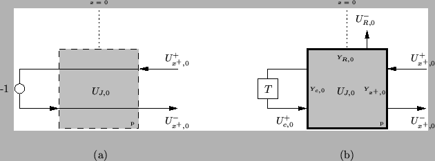The other boundary termination requires a bit more analysis, because we do not have access to $I_{J}$ at a parallel junction. It is sufficient to drop the left hand port entirely in this case (or, equivalently, to terminate the junction with an open circuit, which, when connected in parallel, may be ignored). In this case, though, we must retain the self-loop and the loss/source port. We now show that such a termination does indeed approximate the boundary condition $i(0,t) = 0$. The resulting termination is shown in Figure 4.17(b).

Beginning from system (4.43), where we assume no source (to avoid conflicting conditions at the boundary), we can apply centered differences in time, and use a one-sided [176] approximation for the spatial derivative,

$$\left.\frac{\partial i}{\partial x}\right\vert _{x=0, t = (n+\frac{1}{2})T} = \frac{2}{\Delta}\Big(i({\textstyle \frac{1}{2}},(n+{\textstyle \frac{1}{2}})T)-i(0,(n+{\textstyle \frac{1}{2}})T)\Big) + O(\Delta)\notag$$

$$= \frac{2}{\Delta}i({\textstyle \frac{1}{2}},(n+{\textstyle \frac{1}{2}})T) + O(\Delta)$$

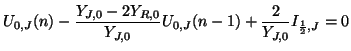
where we have set $i(0,(n+{\textstyle \frac{1}{2}})T) = 0$ in accordance with the boundary condition. This yields the difference approximation to (4.43b) given by

$$U_{0}(n) - \frac{2\bar{c}_{0}-g_{0}T}{2\bar{c}_{0}+g_{0}T}U_{0}(n... ...4}{2v_{0}\bar{c}_{0}+g_{0}\Delta}I_{\frac{1}{2}}(n-{\textstyle \frac{1}{2}})= 0$$ (4.57)

The difference formula obtained from the network termination of Figure 4.17(b) is

$$U_{0,J}(n) - \frac{Y_{J,0}-2Y_{R,0}}{Y_{J,0}}U_{0,J}(n-1)+ \frac{2}{Y_{J,0}}I_{\frac{1}{2},J} = 0$$

where we now have

$$Y_{J,0} \triangleq Y_{x^{+},0}+Y_{R,0}+Y_{c,0}$$ (4.58)

It is easy to see that if we set

$$Y_{R,0} = \frac{1}{2}g_{0}\Delta \hspace{1.0in} Y_{J} = \frac{1}{2}v_{0}\left(2\bar{c}_{0}+g_{0}T\right)$$ (4.59)

then the waveguide network is indeed performing a calculation equivalent to (4.46). $Y_{c,0}$ and $Y_{x^{+},0}$ may be set according to the type of network we are using (i.e., I, II or III in §4.3.6) as long as (4.47) and (4.48) are satisfied; the stability bounds are unchanged. It is important to note that this realization of the boundary condition $i(0,t) = 0$ will be first-order accurate in the grid spacing $\Delta$, due to our use of a one-sided difference approximation. It is recommended, then, to align the waveguide network such that a series junction lies at the left-most grid point, where it can be simply terminated by an open circuit. Such a termination will be second-order accurate.

Because any bounded reflectance may be used to terminate the waveguide network, it has been proposed [96] (in the context of the Karplus-Strong algorithm [103], which can be shown to be equivalent to a particular digital waveguide configuration [168]) that one can model wave propagation in a dispersive medium (like a beam [77]) by using a non-dispersive waveguide for the interior with an all-pass terminating reflectance. Such an all-pass filter will introduce a frequency-dependent phase delay which can be chosen so as to match the dispersion of the medium itself, without dissipating energy. It should be kept in mind, however, that one means of synthesizing such an all-pass filter would be by adding an additional chain of junctions on the opposing side of the boundary junction, and terminating it with an open- or short-circuit. Synthesis (for a given dispersion profile) presumably proceeds along the lines of methods used in related filter-design areas [215].