Boundary Conditions

We now examine the termination of the waveguide mesh which simulates the behavior of the (2+1)D parallel-plate equations. The two most important types of boundary conditions are

$$u =0$$ Short-circuit termination (4.80)

$$i_{n} =0$$ Open-circuit termination (4.81)

where $i_{n}$ refers to the component of $(i_{x},i_{y})$ which is normal to the boundary. Condition (4.68) corresponds to a transmission line plate pair which are connected (and thus short-circuited) at the boundary; the same condition holds for a clamped membrane for which $u$ is interpreted as a transverse velocity, and $(i_{x},i_{y})$ as in-plane forces. Condition (4.69) is an open-circuited termination; current can not leave the plate at the edges. This second condition is analogous to the rigid termination of a (2+1)D acoustic medium, where $(i_{x},i_{y})$ are interpreted as flow velocities, and $u$ as a pressure. Both conditions are of the form of (3.8), and are lossless. We will examine only the termination of the mesh on a rectangular domain (though the result extends easily to the radial mesh to be discussed in §4.6.2).

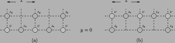
In the case of the (1+1)D transmission line, we could treat a staggered mesh terminated by a parallel junction, and through the duality of $i$ and $u$ extend the result to include termination by a series junction (see §4.3.9). This is no longer the case in (2+1)D, and we must treat the two types of termination separately. Consider a bottom (southern) boundary at $y=0$ of an interleaved mesh of the type shown in Figure 4.21. The two possible types of termination are shown in Figure 4.23.

Figure 4.23: Grid terminations at a southern boundary.