


Next: Grid Arrangement with Normal
Up: Boundary Conditions
Previous: Boundary Conditions
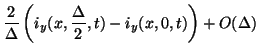
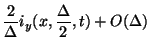
Consider the termination arrangement of Figure 4.23(a). In the source-free case, if for  we have
 , then from (4.58a),
 for for |
|
Thus the current density component tangential to the boundary is uncoupled from the other dependent variables. It is convenient to assume, then, that
 is initially zero, so that it will remain so permanently. In this case, we can drop the series junctions corresponding to
  on the southern boundary from the network. Otherwise, we may allow the junctions to remain, as lumped damped (by a factor
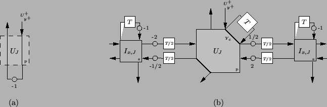
  ) elements, still uncoupled from the rest of the network. In either case, the parallel junctions at the grey points in Figure 4.23(a) may be short-circuited as in the (1+1)D case in order to realize boundary condition (4.68). The waveguide mesh termination corresponding to (4.68) is shown in Figure 4.24(a).
To deal with the boundary condition
 , we may proceed as in the (1+1)D case, and write down a difference approximation to (4.58c), where we use the one-sided difference approximation
and centered differences in the time and  directions,
where
 and
and
 are as given in (4.60).
Here, the voltages on the boundary are related to the tangential currents, which, from Figure 4.23(a), are also calculated on the boundary. This implies that the corresponding junctions will be connected to one another by waveguides which lie directly on the boundary. Also notice the doubled weighting of the  grid function at the boundary; this requires special care in the DWN implementation, though it also follows from a structurally passive termination, provided we make use of transformers along the boundary waveguides. Though we have not discussed transformers in the DWN context [166], they are identical to wave digital transformers, which were mentioned in §2.3.4. In effect, we may introduce multiplies by
  and
and  , for any real in the two signal paths of any waveguide without affecting losslessness, provide we scale impedances at both ends of the waveguide accordingly. The DWN termination corresponding to
  at a southern boundary is shown in Figure 4.24(b). We have used transformers of turns ratio 2, implying that the immittances on the boundary satisfy
 |
(4.82) |
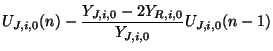
The corresponding difference equation at a parallel boundary junction is then
where
 |
(4.83) |
The junction updating will be equavlent to the centered difference scheme if we choose
 |
(4.84) |
Given that the northward immittances at the boundary junctions must be set as interior values, the settings for the remaining immittances for the type I and II meshes discussed in §4.4.2 will be
Type I:
Type II:
The passivity conditions which follow from the positivity of the boundary self-loop immittances will be
and clearly are less restrictive than the conditions (4.63) and (4.67) over the mesh interior, and hence do not affect the overall stability bound on  .
.
Figure 4.24:
(2+1)D waveguide mesh terminations at a southern boundary, for the grid arrangement of Figure 4.23(a)-- (a) for
and (b)
 .
.
 |
Next: Grid Arrangement with Normal
Up: Boundary Conditions
Previous: Boundary Conditions
Stefan Bilbao
2002-01-22


 Type I
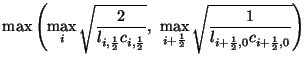 Type II