The Waveguide Mesh in Radial Coordinates

We will look at waveguide meshes in general curvilinear coordinates in §4.8, but radial coordinates are an important special case, especially for musical instrument physical modelling applications (considering how many instruments exhibit some form of radial symmetry).

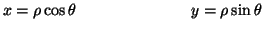
In terms of radial coordinates $(\rho,\theta)$, where

$$x = \rho\cos\theta\hspace{1.0in}y = \rho\sin\theta$$ (4.93)

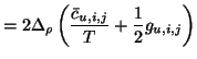
the parallel-plate system (4.58) becomes

$$\begin{eqnarray}l_{\rho}\frac{\partial i_{\rho}}{\partial t} + \f... ...a\frac{\partial i_{\theta}}{\partial \theta} +g_{u}u + e_{u} = 0 \end{eqnarray}$$ (4.94a)

where we define radial and angular current densities by

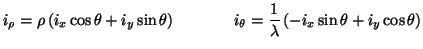$$i_{\rho} = \rho\left(i_{x}\cos\theta+i_{y}\sin\theta\right)\hspac... ...5in}i_{\theta} = \frac{1}{\lambda}\left(-i_{x}\sin\theta+i_{y}\cos\theta\right)$$ (4.95)

and the effective radial material parameters and sources by

$$l_{\rho} = \frac{l}{\rho} l_{\theta} = \rho l\lambda c_{u} = \rho c$$

$$r_{\rho} = \frac{r}{\rho} r_{\theta} =\rho r \lambda g_{u} = \rho g$$ (4.96)

$$e_{\rho} = e\cos\theta+f\sin\theta e_{\theta} =\rho\left(-e\sin\theta+f\cos\theta\right) e_{u} = \rho h$$

$\lambda$ is a scaling coefficient which we will set, in anticipation of discretization, equal to $\frac{\Delta_{\theta}}{\Delta_{\rho}}$, the ratio of the grid spacings in the $\theta$ and $\rho$ directions. We will allow these spacings to be, in general, different.

It is evident that system (4.82) has a form similar to its counterpart in rectilinear coordinates, apart from the extra factor of $\lambda$ in (4.82c). The chief difference is that we now have different effective inductances $l_{\rho}$ and $l_{\theta}$ in the two coordinate directions, but, as we shall see, this anisotropy is easily taken care of (indeed, we could have defined anisotropic inductances $l_{x}$ and $l_{y}$ in the rectilinear case without greatly complicating matters). 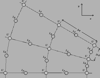We can see immediately that when centered differences are applied to system (4.82), we will be able to operate on an interleaved grid in the $(\rho,\theta)$ coordinates. A version of Yee's algorithm in arbitrary curvilinear coordinates first appeared in [91], and is also discussed in [209]. The interleaved grid, viewed in rectilinear coordinates, is shown in Figure 4.28, where, as before, the dependent variable to be calculated at a particular grid point is indicated next to the point. Grey and white coloring of points indicates operation at alternating time steps.

Figure 4.28: Interleaved grid in radial coordinates.

Centered differencing yields a scheme nearly identical to (4.59), with, again, the difference that the inductance has a directional character. We can thus proceed directly to the waveguide mesh, and, furthermore, can use the same indexing as in the rectilinear case; now, the grid indices $(i,j,n)$ will refer to points $(\rho,\theta,t) = (i\Delta_{r},j\Delta_{\theta},nT)$. Due to the interleaved nature of the resulting difference approximations, we will have series junctions at locations $(i+\frac{1}{2},j,n+\frac{1}{2})$ and $(i, j+\frac{1}{2},n+\frac{1}{2})$ for $i> 0$, $j$ and $n$ integer (with associated junction currents $I_{\rho J,i+\frac{1}{2},j}(n+\frac{1}{2})$ and $I_{\theta J,i,j+\frac{1}{2}}(n+\frac{1}{2})$) and parallel junctions at locations $(i,j,n)$ where we will calculate junction voltages $U_{J,i,j}(n)$, for $i> 0$, $j$ and $n$ integer (we return to the central grid point at $i=0$ later in this section). The computational molecule of the mesh is shown in Figure 4.29.

Figure 4.29: Waveguide mesh for the (2+1)D parallel-plate system, in radial coordinates.

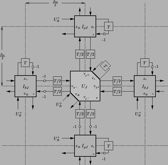Figure 4.30: Representative scattering junctions for the waveguide mesh for the (2+1)D parallel-plate system, in radial coordinates.

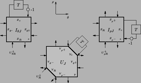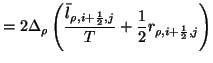
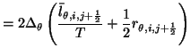
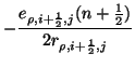
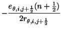
Referring to Figure 4.30, which gives the immittance nomenclature in the waveguide network, and where in addition we have the junction immittances defined by

$$Y_{J,i,j} \triangleq Y_{\rho^{-},i,j}+Y_{\rho^{+},i,j}+Y_{\theta^{+},i,j}+Y_{\theta^{-},i,j}+Y_{c,i,j}+Y_{R,i,j}$$

$$Z_{J,i+\frac{1}{2},j} \triangleq Z_{\rho^{+},i+\frac{1}{2},j}+Z_{\rho^{-},i+\frac{1}{2},j}+Z_{c,i+\frac{1}{2},j}+Z_{R,i+\frac{1}{2},j}$$

$$Z_{J,i,j+\frac{1}{2}} \triangleq Z_{\rho^{+},i,j+\frac{1}{2}}+Z_{\rho^{-},i,j+\frac{1}{2}}+Z_{c,i,j+\frac{1}{2}}+Z_{R,i,j+\frac{1}{2}}$$

for $i> 0$ and $j$ integer, we can perform an analysis similar to the rectilinear case in order to determine that we must have

$$Y_{J,i,j} = 2\Delta_{\rho}\left(\frac{\bar{c}_{u,i,j}}{T}+\frac{1}{2}g_{u,i,j}\right) Y_{R,i,j} = \Delta_{\rho}g_{u,i,j}\notag$$

$$Z_{J,i+\frac{1}{2},j} = 2\Delta_{\rho}\left(\frac{\bar{l}_{\rho,i+\frac{1}{2},j}}{T}+\frac{1}{2}r_{\rho,i+\frac{1}{2},j}\right) Z_{R,i+\frac{1}{2},j} = \Delta_{\rho}r_{\rho,i+\frac{1}{2},j}$$

$$Z_{J,i,j+\frac{1}{2}} = 2\Delta_{\theta}\left(\frac{\bar{l}_{\theta,i,j+\frac{1}{2}}}{T}+\frac{1}{2}r_{\theta,i,j+\frac{1}{2}}\right) Z_{R,i,j+\frac{1}{2}} = \Delta_{\theta}r_{\theta,i,j+\frac{1}{2}}\notag$$

(The junction admittance $Y_{J,0,0}$ will be dealt with shortly.) The source waves should be chosen as

$$U_{R,i,j}^{+}(n) = -\frac{e_{u,i,j}(n)}{2g_{u,i,j}}$$

$$I_{R,i+\frac{1}{2},j}^{+}(n+{\textstyle \frac{1}{2}}) = -\frac{e_{\rho,i+\frac{1}{2},j}(n+{\textstyle \frac{1}{2}})}{2r_{\rho,i+\frac{1}{2},j}}$$

$$I_{R,i,j+\frac{1}{2}}^{+}(n+{\textstyle \frac{1}{2}}) = -\frac{e_{\theta,i,j+\frac{1}{2}}(n+{\textstyle \frac{1}{2}})}{2r_{\theta,i,j+\frac{1}{2}}}$$

where we may of course use the dual type of wave in regions where the loss parameters become small, as discussed in §4.3.7. Just as in the rectilinear case, these conditions define a family of waveguide networks which solve the radial transmission line equations. We here provide the impedance settings for voltage- and current-centered meshes, as well as stability bounds.