The Waveguide Mesh in General Curvilinear Coordinates

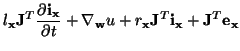
A generalization of the waveguide mesh to arbitrary curvilinear coordinates is useful in that it becomes possible to model boundary conditions which may not be simply aligned with a rectilinear grid. The resulting structure is quite similar to the interleaved forms discussed earlier, and for this reason we will give only a brief description of the coordinate transformation procedure. Consider the following system:

$$\begin{eqnarray}l_{{\bf x}}\frac{\partial {\bf i_{x}}}{\partial t... ...a_{{\bf x}} \cdot {\bf i_{x}} + g_{{\bf x}}u + h_{{\bf x}} &=& 0 \end{eqnarray}$$ (4.113a)

Here we may assume any number $k$ of physical spatial coordinates ${\bf x} = [x_{1}, \hdots, x_{k}]^{T}$, so that $\nabla_{{\bf x}} = \frac{\partial}{\partial {\bf x}} = [\frac{\partial}{\partial x_{1}},\hdots, \frac{\partial}{\partial x_{k}}]^{T}$. ${\bf i_{x}}$ and ${\bf e_{x}}$ are both assumed to be $k$-dimensional column vectors. $l_{{\bf x}}$, $c_{{\bf x}}$, $r_{{\bf x}}$ and $g_{{\bf x}}$ are all positive functions of ${\bf x}$ ( $l_{{\bf x}}$ and $c_{{\bf x}}$ are strictly positive), and ${\bf e_{x}}$ and $h_{{\bf x}}$ are the source terms. If $k$ is 1 or 2, then we have the transmission line or parallel-plate transmission line system respectively, and if $k=3$, we have the system describing linear acoustic phenomena (assuming that the material parameters are constant).

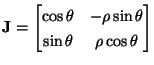
Consider the mapping

$${\bf x} = \mbox{\boldmath$\zeta$} ({\bf w})$$

where ${\bf w} = [w_{1}, \hdots, w_{k}]^{T}$ are the transformed coordinates. A rectilinear grid in the ${\bf w}$ coordinates can be mapped to a curvilinear grid in the physical ${\bf x}$ coordinates. We can then define the $k\times k$ matrix of partial derivatives ${\bf J}$ by

$$[{\bf J}_{\alpha,\beta}] = \frac{\partial\zeta_{\alpha}}{\partial w_{\beta}}\hspace{0.5in}\alpha,\,\beta = 1,\hdots,k$$

where $\zeta_{\alpha}$ is the $\alpha$th component of $\zeta$. We assume ${\bf J}$ to be nonsingular everywhere in the problem domain (though this assumption may be relaxed as will mention later in this section) . Defining the differential operator $\nabla_{{\bf w}}$ by $\nabla_{{\bf w}} = \frac{\partial}{\partial {\bf w}} = [\frac{\partial}{\partial w_{1}},\hdots, \frac{\partial}{\partial w_{k}}]^{T}$, it then follows [69] that

$$\nabla_{{\bf w}} = {\bf J}^{T}\nabla_{{\bf x}}\hspace{0.5in}\nabl... ... J}\vert}\nabla_{{\bf w}}\cdot\left(\vert{\bf J}\vert{\bf J}^{-1}{\bf a}\right)$$

for any $k\times 1$ column vector ${\bf a}$. Here, $\vert{\bf J}\vert$ is the so-called Jacobian determinant [172]. Using these relationships, the system (4.97) may be rewritten as

$$l_{{\bf x}}{\bf J}^{T}\frac{\partial {\bf i_{x}}}{\partial t}+\nabla_{{\bf w}}u + r_{{\bf x}}{\bf J}^{T}{\bf i_{x}}+{\bf J}^{T}{\bf e_{x}} = {\bf0}$$

$$c_{{\bf x}}\vert{\bf J}\vert\frac{\partial u}{\partial t}+\nabla_... ...{\bf i_{x}}\right)+\vert{\bf J}\vert g_{{\bf x}}u+\vert{\bf J}\vert h_{{\bf x}} = 0 \$$

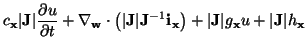
or

$$\begin{eqnarray}{\bf L_{w}}\frac{\partial {\bf i_{w}}}{\partial t... ...bla_{{\bf w}}^{T}\cdot{\bf i_{w}}+g_{{\bf w}}u+h_{{\bf w}} &=& 0 \end{eqnarray}$$ (4.114a)

where

$${\bf i_{w}} = \vert{\bf J}\vert{\bf J}^{-1}{\bf i_{x}}$$

and

$${\bf L_{w}} = \frac{l_{{\bf x}}}{\vert{\bf J}\vert}{\bf J}^{T}{\bf J} {\bf R_{w}} = \frac{r_{{\bf x}}}{\vert{\bf J}\vert}{\bf J}^{T}{\bf J} {\bf e_{w}} = {\bf J}^{T}{\bf e_{x}}$$

$$c_{{\bf w}} = \vert{\bf J}\vert c_{{\bf x}} g_{{\bf w}} = \vert{\bf J}\vert g_{{\bf x}} h_{{\bf w}} = \vert{\bf J}\vert h_{{\bf x}}$$

System (4.98) is similar to (4.97), except that we now have ``vector'' inductance and resistance coefficients (note that both ${\bf L_{w}}$ and ${\bf R_{w}}$ are positive definite matrices, if ${\bf J}$ is non-singular). In particular, it is still symmetric hyperbolic (see §3.2), so we may expect that it is possible to derive a waveguide structure.

Consider now the transformed system (4.98) in (2+1)D. If ${\bf J}^{T}{\bf J}$ is diagonal, then ${\bf L_{w}}$ and ${\bf R_{w}}$ will be as well; in this case, system (4.98) is in the same form as the parallel-plate system in radial coordinates (4.82), so we need not discuss this case further here. Indeed, the radial system is a special case of (4.98) with ${\bf w} = [\rho, \theta]^{T}$ and

$${\bf J} = \begin{bmatrix}\cos\theta&-\rho\sin\theta\\ \sin\theta&\rho\cos\theta\\ \end{bmatrix}$$

On the other hand, if ${\bf J}^{T}{\bf J}$ is not diagonal (so that we are working in non-orthogonal or oblique coordinates), then the situation is more complex. Due to the cross-coupling between the components of ${\bf i_{w}}$ through the matrices ${\bf L_{w}}$ and ${\bf R_{w}}$, it will no longer be possible to stagger all the components of the solution; in particular, it will be necessary to use vector scattering junctions. Let us look at the case $k=2$, so that (4.98) are the equations of the parallel-plate system in the curvilinear coordinates ${\bf w}$. Furthermore, we will set $w_{1} = p$ and $w_{2} = q$. A centered difference approximation to (4.98), over grid points with coordinates $p=i\Delta$ and $q=j\Delta$, and at times $t = nT$ for $i$, $j$ and $n$ half-integer is

$$\begin{eqnarray}v_{0}\bar{{\bf L}}_{{\bf w},i+\frac{1}{2},j}\Big(... ...ac{\Delta}{2}\Big(h_{{\bf w},i,j}(n)+h_{{\bf w},i,j}(n-1)\Big)=0 \end{eqnarray}$$

Here, we have the vector grid function ${\bf I}_{i+\frac{1}{2},j}(n+{\textstyle \frac{1}{2}})$, which is a two-vector with components $I_{p,i+\frac{1}{2},j}(n+{\textstyle \frac{1}{2}})$ and $I_{q,i+\frac{1}{2},j}(n+{\textstyle \frac{1}{2}})$ as well as the scalar grid function $U_{i,j}(n)$. $\bar{{\bf L}}_{{\bf w},i+\frac{1}{2},j+\frac{1}{2}}$ and $\bar{c}_{{\bf w},i,j}$ are second-order approximations to ${\bf L}_{{\bf w}}$ and $c_{{\bf w}}$ at the indicated grid points. The scheme above has been written so that it is clear that it can operate for $n$ integer, and for $i$ and $j$ such that $i+j$ is integer; notice that $U$ and ${\bf I}$ are calculated at alternating time instants and grid locations, but the components of ${\bf I}$ can not, in general, be calculated at separate locations. $v_{0}$, again, is equal to $\Delta/T$, and (4.99) will be a second-order accurate approximation to (4.98).

We will skip the tedious procedure of deriving a waveguide mesh, and simply present the resulting structure in Figure 4.34.

Figure 4.34: (2+1)D DWN for the parallel-plate system (4.98) in general non-orthogonal curvilinear coordinates.

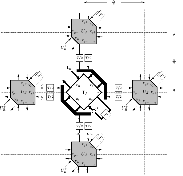Junction vector currents ${\bf I}_{J}$ are calculated at the series vector scattering junctions; the black bars surrounding this junction in the figure are the splitting elements that were discussed in §4.2.6. Although we have not drawn them in the figure, there will be similar vector junctions at the four grid points neighboring any of the parallel junctions where the voltages $U_{J}$ are calculated. This vector junction has four $2\times 2$ matrix impedances associated with it: ${\bf Z}_{c}$, the self-loop impedance, ${\bf Z}_{R}$, the loss/source impedance, and ${\bf Z}_{1}$ and ${\bf Z}_{2}$, which are constrained (see §4.2.6) to be

$${\bf Z}_{1, i+\frac{1}{2},j} = \begin{bmatrix}\frac{1}{Y_{p^{+},i... ...},i+1,j}}&0\\ 0&\frac{1}{Y_{q^{-},i+\frac{1}{2},j+\frac{1}{2}}}\\ \end{bmatrix}$$ (4.116)

The junction impedance ${\bf Z}_{J}$ is defined to be the sum of these four matrices. The admittances at the parallel junctions are defined in a manner similar to those of the DWN in rectilinear coordinates. Also, we have the source voltage waves $U^{+}_{R,i,j}$ at the parallel junctions and vector source current waves ${\bf I}^{+}_{R,i+\frac{1}{2},j}$ at the series junctions.

This DWN can be identified with the difference system (4.99) if we set

$${\bf Z}_{J} = 2v_{0}\bar{{\bf L}}_{{\bf w}}+\Delta{\bf R}_{{\bf w}} {\bf Z}_{R} = \Delta{\bf R}_{{\bf w}} {\bf I}_{R}^{+} = -\Delta{\bf R}_{{\bf w}}^{-1}{\bf e}_{{\bf w}}/2$$

$$Y_{J} = 2v_{0}\bar{c}_{{\bf w}}+\Delta g_{{\bf w}} Y_{R} = \Delta g_{{\bf w}} U_{R}^{+} = -\Delta g_{{\bf w}}h_{{\bf w}}/2$$

at the grid points for which such quantities are defined.

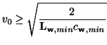
There are, of course, various realizations, depending on how the self-loop and connecting immittances are chosen. First, note that because ${\bf Z}_{J}$ is not diagonal, it will not be possible to distribute it equally among the two connecting impedances ${\bf Z}_{1}$ and ${\bf Z}_{2}$, which are constrained to be diagonal from (4.100). Thus a type II (current-centered) realization analogous to that which was discussed in the case of the rectilinear mesh will not be possible, even in the absence of losses and sources. A type I realization is certainly possible, but for brevity sake, we will only provide the settings for the type III DWN. Here all the connecting impedances are all set to be some constant value $Z_{const}$. This then implies that

$${\bf Z}_{c} = 2v_{0}\bar{{\bf L}}_{{\bf w}} - 2Z_{const}{\bf I}_{2}\hspace{0.5in}Y_{c} = 2v_{0}\bar{c}_{{\bf w}}-4/Z_{const}$$

where ${\bf I}_{2}$ is the $2\times 2$ identity matrix. Requiring the positivity of $Y_{c}$ and the positive definiteness of ${\bf Z}_{c}$ gives the constraint

$$v_{0}\geq \sqrt{\frac{2}{{\bf L}_{{\bf w}, min}c_{{\bf w},min}}}$$

for $c_{{\bf w},min}$ the minimum of $c_{{\bf w}}$ over parallel junction locations and ${\bf L}_{{\bf w},min}$ the minimum of the eigenvalues of ${\bf L}_{{\bf w}}$ over series junction locations, and where we have made the choice

$$Z_{const} = \sqrt{\frac{2{\bf L}_{{\bf w}, min}}{c_{{\bf w},min}}}$$

In general, this bound will depend on the choice of coordinates.

FDTD in general curvilinear coordinates has developed in a similar way; most formulations are slightly different in that they are based on a tensor density formulation [91,209] and employ a double set of variables (covariant and contravariant) in the non-orthogonal case; differencing involves interleaving these two sets of components at alternating time steps. They have also been used as a starting point for developing FDTD methods in ``local'' coordinates defined with respect to an automatically generated grid [72,73]. Curvilinear coordinate systems have been touched upon in the MDWD framework as well; An approach similar to the above is discussed in [69], and a tensor density formulation is given in [131].