In this brief section we summarize, for completeness sake, (3+1)D waveguide meshes, introduced in [200] and [156]. We will return to these mesh formulations in §4.9.5, where we will discuss interfaces between meshes of different grid densities. We will also analyze the spectral characteristics of these methods in some detail in Appendix A.
The transmission line problem with spatially-varying material parameters does not generalize in a meaningful way to (3+1)D; there is no commonly-known physical system that would behave according to such a set of equations (though linear acoustics in non-Cartesian coordinates might serve as one example). Physical systems of interest in (3+1)D generally have a more complex form than would be implied by such a straightforward generalization. We will have occasion to examine two such systems in detail, namely the (3+1)D equations describing the vibration of a linear, isotropic elastic solid, in §5.6, and Maxwell's equations (see §4.10.6).
The (3+1)D wave equation, however, is of interest in linear acoustics (and it is arrived at by linearizing a system of conservation laws, namely Euler's equations [112], to which we will return briefly in Appendix B). It is written as
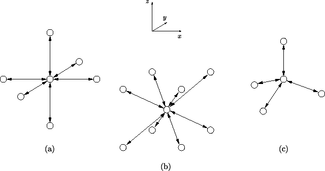
Three regular grids are shown in Figure 4.33, and we have indicated waveguide couplings between neighboring points (where scattering junctions will be placed) by double-headed arrows. Delays in these bidirectional delay lines are assumed to be of length ![]() , and are identical over the entire network, in all three cases. Junctions are separated by a distance
, and are identical over the entire network, in all three cases. Junctions are separated by a distance ![]() . The first, shown in (a), is the standard rectilinear mesh [156,198], and the second, shown in (b) is a mesh obtained by superimposing one rectilinear grid on top of a shifted copy of itself, then connecting each point to its eight nearest neighbors; an appropriate name for such a configuration might be an ``octahedral mesh.'' A third structure, the so-called tetrahedral mesh [200], is shown in (c). Self-loops, necessary when we are operating away from the CFL bound, are not shown, and the immittances of the connecting waveguides are assumed to all be identical. Other structures are also conceivable.
. The first, shown in (a), is the standard rectilinear mesh [156,198], and the second, shown in (b) is a mesh obtained by superimposing one rectilinear grid on top of a shifted copy of itself, then connecting each point to its eight nearest neighbors; an appropriate name for such a configuration might be an ``octahedral mesh.'' A third structure, the so-called tetrahedral mesh [200], is shown in (c). Self-loops, necessary when we are operating away from the CFL bound, are not shown, and the immittances of the connecting waveguides are assumed to all be identical. Other structures are also conceivable.
We remark here on a computational aspect of these junctions--as mentioned in [200], if we are at CFL (and so do not need self-loops), it is useful to have the number of waveguides connected to a particular junction be a power of two; if this can be arranged, then all multiplies carried out during the scattering step may be implemented as simple bit-shifting operations in a fixed-point implementation. Because this is not true for the rectilinear mesh, (i.e., there are six waveguides connected to each junction), the tetrahedral mesh was proposed as a more efficient structure. We note, however, that the octahedral mesh, with eight waveguides connected to each junction, also can be implemented efficiently in fixed-point. Furthermore, it may be easier to deal with from the programmer's point of view, because unlike the tetrahedral mesh, it will not involve any special indexing strategy (for a tetrahedral mesh, half of the junctions will have an inverse orientation with respect to the other half).
If we are at the CFL bound--that is if we have
| Rectilinear mesh | ||||
 |
Octahedral mesh | |||
| Tetrahedral mesh |