Grid Density Doubling in (3+1)D

It is straightforward to extend the grid density doubling technique presented in §4.9.1 to (3+1)D. As in §4.7, we will assume that our mesh is to simulate the (3+1)D wave equation (4.95).

Figure 4.43: (a) Grid $I$, with grid spacing $\Delta$, is adjoined to a doubled density region $II$ with grid spacing $\frac{\sqrt{3}\Delta}{2}$. (b) a junction at the interface.

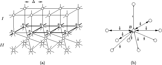If we have a rectilinear mesh (region $I$ in Figure 4.43(a)) with inter-junction spacing $\Delta$ to which we would like to adjoin a mesh of doubled grid density, we may introduce an octahedral mesh (region $II$) with a grid spacing of $\sqrt{\frac{3}{4}}\Delta$, to be connected to region $I$ across an interface; special matching waveguide connections at this interface are shown in bold in Figure 4.43(a). The spacing of $\sqrt{\frac{3}{4}}\Delta$ in region $II$ is chosen so that the octahedral grid may be decomposed into two offset rectilinear grids of spacing $\Delta$, and may hence be aligned with region $I$ at the interface.

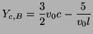
The relative admittances at the special boundary 10-ports (nine connecting waveguides and a self-loop) are shown in Figure 4.43(b); only the waveguides in bold in (a) take on special values; all others may be set as interior admittances. For consistency with the wave equation, we must choose the admittances in region $I$ to be double those in region $II$. In addition, the self-loop admittance at a boundary junction (labelled $B$ in Figure 4.43) must be chosen to be

$$Y_{c,B} = \frac{3}{2}v_{0}c-\frac{5}{v_{0}l}$$

where we have chosen the connecting admittance in region $I$ to be $\frac{1}{v_{0}l}$, and where we must have $\gamma = \sqrt{\frac{1}{lc}}$ as discussed in §4.7. The stability requirement at such a boundary junction $B$ is then

$$v_{0}\geq \sqrt{\frac{10}{3}}\gamma$$

which is worse than the bound over the interior of region $I$, as given in (4.96). On the other hand, because the grid spacing is $\sqrt{\frac{3}{4}}\Delta$ in region $II$, we must set, at an interior point in region $II$,

$$Y_{c} = cv_{0}-\frac{4}{v_{0}l}\hspace{0.5in}\Rightarrow\hspace{0.5in} v_{0}\geq 2\gamma \mbox{{\rm in region $II$}}$$

This bound is, as expected, worse still than the boundary requirement, and hence boundary scattering, as in the (2+1)D case, does not compromise the overall requirement on space step/time step ratio which is forced by the settings in region $II$.

We briefly mention that at edges and corners of a doubled density region, the waveguide mesh cannot be made consistent with the wave equation. We may invoke the same argument that was ventured in the (2+1)D case, namely that numerical reflection should be minimal, and should vanish in the limit as the grid spacing becomes small. Special admittance values for the connecting waveguides along such edges, and for the self-loops at both edges and corners may be chosen such that numerical reflection is made as small as possible, though we do not provide here those values, due to the ease with which they can be calculated, and relatively large number of cases that must be considered (two edge types and four corner types).

We have not investigated ways of redoubling (quadrupling) grid density as was done in the (2+1)D case, though we would conjecture that it should be possible, either via a direct quadrupling layer with a special interface (analogous to the scheme of §4.9.3) or via successive redoubling (as per §4.9.2).