As a simple application of an interface between radial and rectilinear meshes, we solve the (2+1)D acoustic wave equation (1.18) in a U-shaped tube--that is, a tube consisting of two straight segments connected by a semicircular radial tube; we note that the (3+1)D version of this problem was first solved using a waveguide mesh by Tim Stilson at CCRMA, in the context of physical modeling of brass instruments [200]. In that case, a rectilinear mesh was used over the entire domain, which forces a staircase-type approximation to the radial boundary. Here, however, because we are modeling the semicircular tube in radial coordinates, boundary conditions can be implemented in a well-defined manner; the trade-off will be in the added numerical reflection at the radial/rectilinear mesh interface.
We assume a wave speed of 1 throughout the interior, and an open-circuited boundary condition (![]() , the normal current density component is zero everywhere on the boundary). The thickness of the tube is 0.2, the inner radius of the circular portion is 0.1, and the lengths of the two straight tube segments are each 0.3. The grid spacing is set to
, the normal current density component is zero everywhere on the boundary). The thickness of the tube is 0.2, the inner radius of the circular portion is 0.1, and the lengths of the two straight tube segments are each 0.3. The grid spacing is set to
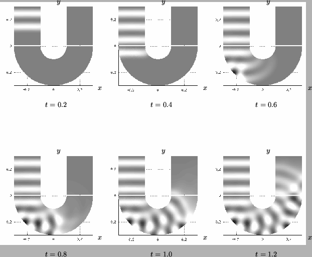
![]() , and white lines indicate the interfaces between the radial mesh and the adjacent rectilinear meshes. The input signal is a raised cosine voltage of period 0.2 at the upper left-hand entrance to the tube. The evolution of the voltage in the tube is shown in Figure 4.42. Here,
, and white lines indicate the interfaces between the radial mesh and the adjacent rectilinear meshes. The input signal is a raised cosine voltage of period 0.2 at the upper left-hand entrance to the tube. The evolution of the voltage in the tube is shown in Figure 4.42. Here, ![]() can be interpreted as a pressure in a tube with hard boundaries; this situation comes up in the modelling of brass instruments, in particular in curved sections of tubes, such as trombone slides or crooks (though we have used, for illustrative purposes, an unnaturally short wavelength; longer wavelengths in the musical range can be modeled more cheaply using a coarse grid, and numerical reflections will be even smaller as the number of grid points per wavelength increases).
can be interpreted as a pressure in a tube with hard boundaries; this situation comes up in the modelling of brass instruments, in particular in curved sections of tubes, such as trombone slides or crooks (though we have used, for illustrative purposes, an unnaturally short wavelength; longer wavelengths in the musical range can be modeled more cheaply using a coarse grid, and numerical reflections will be even smaller as the number of grid points per wavelength increases).