Next: Simulation: Solving the Acoustic
Up: Interfaces Between Grids
Previous: Grid Density Quadrupling
Connecting Rectilinear and Radial Grids
As another example of a passive interface between different types of waveguide meshes, we examine the means by which grids defined in different coordinate systems may be connected, for the special (but quite practically important) case of the connection between a rectilinear and radial grid. Such a grid would be useful in cases where it is desired to solve the parallel-plate system or wave equation over some region which has boundaries which are are straight in some places, but circularly curved in others. One could in general proceed by attempting to find a global coordinate transformation which maps an irregular region to a regular one (like a rectangle), and then developing a waveguide mesh in the new coordinates, as per the methods discussed in §4.8. It is perhaps simpler, however, to use rectilinear and radial meshes at appropriate places in the domain, and then define a matching layer at the boundary between the regions, which should also be locally consistent with the equations to be solved. Consider the grid arrangement of Figure 4.41.
Figure 4.41:
Interface between radial and rectilinear meshes.
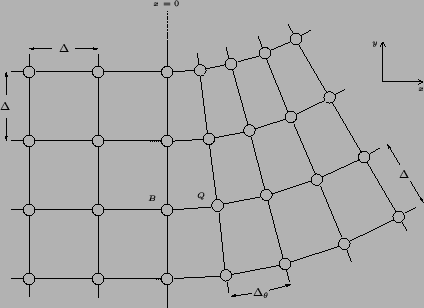 |
We have a type II radial waveguide mesh in  and a type II rectilinear mesh in
  ; parallel junctions are to be placed at all the grid points, and waveguide connections (bidirectional delay lines of delay
  ) are indicated by connecting lines. Special boundary waveguides, which lie along the
  axis, are drawn in bold. All interior waveguide admittances in either region (i.e., all admittances except for those of the boundary waveguides) are assumed to be set to the values that they must take in the interior in order to solve the lossless source-free transmission line equations, as given in (4.64)--(4.66) and (4.89)--(4.92). Self-loops are of course required in general at all junctions, though for simplicity, they are not represented in Figure 4.41. The spacing
  between junctions in the rectilinear mesh is assumed to be equal to the radial grid spacing in the radial mesh. The angular spacing in this same grid,
 , may be set independently. We will use
 here.
here.
In order to derive the admittance and self-loop settings at the boundary, we may examine a junction at coordinates
 ,
,  integer (one such point is labelled
  in Figure 4.41). In keeping with the notation for a rectilinear mesh (used in ), we call the admittances of the four connecting waveguides at such a point
 ,
,
 ,
,
 and
and
 , and the self-loop admittance
  . The junction admittance
  is then the sum of these five admittances. The junction voltage at point will be called
  , and we will call the junction voltage at point
  directly to the right
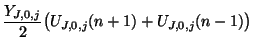
  . The difference scheme in the junction voltages resulting from such a mesh is then
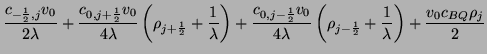
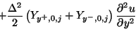
Expansion in terms of a Taylor series about
 gives, in terms of the continuous function
  ,
,
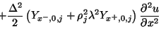
where we have discarded higher-order terms in , and used
 and
and  as in §4.6.2.
First examine, in (4.103), the coefficient of
 on the right-hand side. Notice that in order for this term to behave as
 , we must have
 . Since
is assumed set as an interior admittance in the type II radial waveguide mesh, namely, from (4.90) as
. Since
is assumed set as an interior admittance in the type II radial waveguide mesh, namely, from (4.90) as
where  is the value of the inductance at the midpoint of the waveguide connecting points and , we may choose
Because
is to be interpreted as an interior admittance in the rectilinear mesh, it is clear that all connecting admittances in this mesh should incorporate this same scaling factor of  .
.
Since a boundary waveguide can be interpreted as lying in both waveguide meshes, a good initial guess as to its admittance might be a simple linear average of the admittances of interior radial and rectilinear waveguides located at the same position. This would give:
It is straightforward (but tedious) to show that these admittances do indeed yield a difference scheme which is consistent with the lossless source-free parallel-plate system, provided that we set
where  is the capacitance at the midpoint of the waveguide joining points and , for any . The stability bound is identical to that obtained in the interior of the radial mesh, and this type of matching layer requires very little extra programming effort in an implementation
.
is the capacitance at the midpoint of the waveguide joining points and , for any . The stability bound is identical to that obtained in the interior of the radial mesh, and this type of matching layer requires very little extra programming effort in an implementation
.
Subsections
Next: Simulation: Solving the Acoustic
Up: Interfaces Between Grids
Previous: Grid Density Quadrupling
Stefan Bilbao
2002-01-22