Central Gridpoint in a Radial Mesh

We have so far restricted our attention to interior points of the grid (for which $i> 0$). If the center of the $(\rho,\theta)$ coordinate system is to be contained in the grid, a special treatment is required. We have indexed the grid variables such that, in our interleaved mesh, a single parallel junction lies at the origin (for $i=0$). 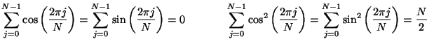If the problem domain includes a full circle, we also must assume that $\Delta_{\theta}$ divides 2$\pi$ evenly so that we have a positive integer $N$ such that

$$N = \frac{2\pi}{\Delta_{\theta}}$$

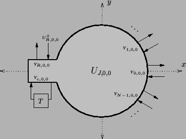
Thus the central parallel junction will be connected to $N$ series junctions at locations $(\frac{\Delta_{\rho}}{2},j\Delta_{\theta})$, $j=0,\hdots, N-1$. We will name the admittances of the $N$ waveguides radiating from the central hub $Y_{j,0,0}$, $j=0,\hdots, N-1$, and the admittance of the self-loop and loss/source ports will be $Y_{c,0,0}$ and $Y_{R,0,0}$ respectively (see Figure 4.31).

Figure 4.31: Central scattering junction for the waveguide mesh in radial coordinates.

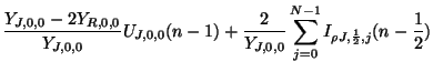
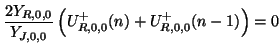
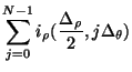
The difference scheme relating the junction voltage at the central grid point to the radial currents at the surrounding junctions will then be

$$U_{J,0,0}(n) - \frac{Y_{J,0,0}-2Y_{R,0,0}}{Y_{J,0,0}}U_{J,0,0}(n-1) + \frac{2}{Y_{J,0,0}}\sum_{j=0}^{N-1}I_{\rho J,\frac{1}{2},j}(n-\frac{1}{2})\notag$$ (4.105)

$$- \frac{2Y_{R,0,0}}{Y_{J,0,0}}\left(U_{R,0,0}^{+}(n)+U_{R,0,0}^{+}(n-1)\right) = 0$$ (4.106)

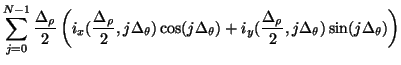
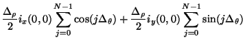
The sum over the junction currents, which we now look at in the continuous time/space domain so as to develop a series approximation) may be rewritten using (4.83) in terms of the rectilinear current variables as

$$\sum_{j=0}^{N-1}i_{\rho}(\frac{\Delta_{\rho}}{2},j\Delta_{\theta}) = \sum_{j=0}^{N-1}\frac{\Delta_{\rho}}{2}\left(i_{x}(\frac{\Delta_{... ...y}(\frac{\Delta_{\rho}}{2},j\Delta_{\theta})\sin(j\Delta_{\theta})\right)\notag$$ (4.107)

$$= \frac{\Delta_{\rho}}{2}i_{x}(0,0)\sum_{j=0}^{N-1}\cos(j\Delta_{\t... ...)+\frac{\Delta_{\rho}}{2}i_{y}(0,0)\sum_{j=0}^{N-1}\sin(j\Delta_{\theta})\notag$$ (4.108)

$$\hspace{0.3in}+\hspace{0.1in} \frac{\Delta_{\rho}^{2}}{4}\sum_{j=... ...tial y}\right\vert _{(0,0)}\hspace{-0.1in}\sin^{2}(j\Delta_{\rho})\right)\notag$$ (4.109)

$$= \frac{N\Delta_{\rho}^{2}}{8}\left(\left.\frac{\partial i_{x}}{\pa... ...pace{-0.1in}+\left.\frac{\partial i_{y}}{\partial y}\right\vert _{(0,0)}\right)$$ (4.110)

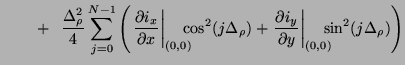
where we have neglected higher order terms in $\Delta_{\rho}$ and used, in the last line, the identities

$$\sum_{j=0}^{N-1}\cos\left(\frac{2\pi j}{N}\right) = \sum_{j=0}^{N... ...}{N}\right)=\sum_{j=0}^{N-1}\sin^{2}\left(\frac{2\pi j}{N}\right) = \frac{N}{2}$$

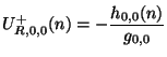
which hold for $N>2$. Using approximation (4.94) and by comparing (4.93) with (4.82c), we must choose the junction and loss/source port admittance to be

$$Y_{J,0,0} = \frac{1}{4}N\Delta_{\rho}^{2}\left(\frac{\bar{c}_{0,0... ...{0,0}}{2}\right)\hspace{0.5in} Y_{R,0,0} = \frac{1}{8}N\Delta_{\rho}^{2}g_{0,0}$$

and the source wave variable $U_{R,0,0}^{+}(n)$ to be

$$U_{R,0,0}^{+}(n) = -\frac{h_{0,0}(n)}{g_{0,0}}$$

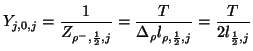
A mesh of type I is infeasible because it would require access to $l_{\rho,0,0}$ in order to set $Z_{c,\frac{1}{2},j}$ as prescribed in (4.86), but $l_{\rho}$ as defined in (4.84) is singular at the origin (although if we are working with a radial geometry which does not contain the origin, this problem does not arise). For a mesh of type II, we have, from (4.89),

$$Y_{j,0,j} = \frac{1}{Z_{\rho^{-},\frac{1}{2},j}} = \frac{T}{\Delta_{\rho}l_{\rho,\frac{1}{2},j}} = \frac{T}{2l_{\frac{1}{2},j}}$$

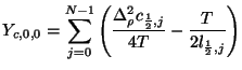
and so we may set, for the self-loop admittance at the central junction,

$$Y_{c,0,0} = \sum_{j=0}^{N-1}\left(\frac{\Delta_{\rho}^{2}c_{\frac{1}{2},j}}{4T} - \frac{T}{2l_{\frac{1}{2},j}}\right)$$

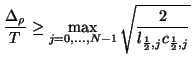
which is positive when

$$\frac{\Delta_{\rho}}{T}\geq \max_{j=0,\hdots,N-1} \sqrt{\frac{2}{l_{\frac{1}{2},j}c_{\frac{1}{2},j}}}$$

Thus the stability requirement at the central junction does not interfere with the requirements over the interior of the mesh given for the type II mesh.

We note that a different type of central node, proposed for use in radial TLM simulations, is described in [24].