Balanced Forms

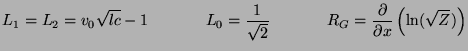
Consider again the (1+1)D transmission line, with spatially-varying coefficients. It has been noted in the past [130,131] that the restriction on the time step, namely

$$v_{0}\geq \frac{1}{\sqrt{l_{min}c_{min}}}$$

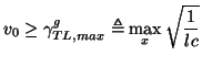
with $l_{min} = \min_{x}l$ and $c_{min} = \min_{x}c$ is rather unsatisfying; the local group velocity at any point in our domain is given by $\pm 1/\sqrt{lc}$, so we would hope that a more physically meaningful bound such as

$$v_{0}\geq \gamma_{TL,max}^{g} \triangleq \max_{x}\sqrt{\frac{1}{lc}}$$ (3.93)

(which is obtained in using, for example, digital waveguide networks, which will be discussed in Chapter 4) could be attainable. Depending on the variation in $l$ and $c$, the new bound can allow a substantially larger time step. We will show that this is in fact possible via a MDWD approach.

The transmission line equations given in (3.56) can be transformed in the following way: first introduce new dependent variables

$$\tilde{i}_{1} = \sqrt{Z}i\hspace{1.0in}\tilde{i}_{2} = u/\sqrt{Z}$$

where $Z$, the local line impedance is defined by

$$Z(x) \triangleq \sqrt{\frac{l}{c}}$$

Such a transformation in fact changes to variables which both have units of root power. After a few elementary manipulations (namely scaling (3.56a) by $1/\sqrt{Z}$ and (3.56b) by $\sqrt{Z}$), we have

$$\begin{eqnarray}\sqrt{lc}\frac{\partial \tilde{i}_{1}}{\partial t... ...{\rm ln}(\sqrt{Z}))\tilde{i}_{1}+gZ\tilde{i}_{1}+h\sqrt{Z} &=& 0 \end{eqnarray}$$ (3.94a)

System (3.91) is still symmetric hyperbolic; referring to the general system from (3.1), for ${\bf w} = [\tilde{i}_{1}, \tilde{i}_{2}]^{T}$, we now have

$${\bf P} = \begin{bmatrix}\sqrt{lc}&0\\ 0&\sqrt{lc}\\ \end{bmatrix... ...frac{\partial}{\partial x}({\rm ln}(\sqrt{Z}))&gZ\\ \end{bmatrix}\hspace{0.2in}$$ (3.95)

Note that because ${\bf P}$ is now a multiple of the identity matrix, there is near complete symmetry between the variables $\tilde{i}_{1}$ and $\tilde{i}_{2}$. We use the term ``balanced'' to describe such a system. Note also that new off-diagonal terms have appeared in ${\bf B}$ (compare (3.92) with (3.57)), but they appear antisymmetrically, and thus do not give rise to loss--in other words these terms do not appear in $({\bf B}+{\bf B})^{T}$, which determines the growth or decay of the solution, as per (3.5). In fact, these off-diagonal terms yield a lossless (but non-reciprocal) gyrator in the circuit setting.

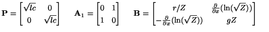
In terms of the coordinates defined by (3.18), we can then rewrite (3.91) as

$$L_{1}D_{t'}\tilde{i}_{1}+L_{0}D_{1}\left(\tilde{i}_{1}+\tilde{i}_... ...i}_{1}-\tilde{i}_{2}\right)+R_{G}\tilde{i}_{2}+\tilde{r}\tilde{i}_{1}+\tilde{e} =$$ 0

$$L_{2}D_{t'}\tilde{i}_{2}+L_{0}D_{1}\left(\tilde{i}_{2}+\tilde{i}_... ...i}_{2}-\tilde{i}_{1}\right)-R_{G}\tilde{i}_{1}+\tilde{g}\tilde{i}_{2}+\tilde{h} =$$ 0

where

$$L_{1}=L_{2}= v_{0}\sqrt{lc}-1\hspace{0.5in}L_{0} = \frac{1}{\sqrt... ...hspace{0.5in}R_{G} = \frac{\partial}{\partial x}\left({\rm ln}(\sqrt{Z})\right)$$

(which should be compared with (3.63), for the standard form), and

$$\tilde{r} = r/Z\hspace{0.2in} \tilde{e} = e/\sqrt{Z}\hspace{0.2in}\tilde{g} = gZ\hspace{0.2in} \tilde{h} = h\sqrt{Z}$$

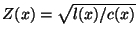
As mentioned previously, in a MDKC setting, the terms with coefficient $R_{G}$ can be treated as a gyrator. The network and its wave digital counterpart are shown in Figure 3.23. The port resistances are given by

$$R_{1} = R_{2} = \frac{2}{\Delta}\left(v_{0}\sqrt{lc}-1\right)\hsp... ...hspace{0.3in}R_{\tilde{er}} = \tilde{r}\hspace{0.3in}R_{\tilde{gh}} = \tilde{g}$$

Figure 3.23: (a) Balanced MD-passive network for the (1+1)D transmission line equations and (b) its associated MDWD network.

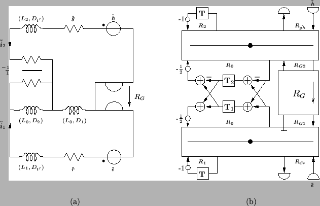In order to accommodate the gyrator, we have been forced, in order to avoid delay-free loops, to set one of the ports to which it is connected to be reflection-free (see §2.3.5). In (1+1)D, we can choose either of these ports, but picking the bottom port in Figure 3.23(b) allows us to extend the idea to (2+1)D easily. This port resistance is then constrained to be

$$R_{G1} = R_{1}+R_{\tilde{er}}+R_{0}$$

We have two simplifying choices for $R_{G2}$; either we can choose it to be reflection-free as well, so that we will have a general gyrator described by (2.25), or we can choose

$$R_{G2} = \frac{R_{G}^{2}}{R_{G1}}$$

in which case the gyrator equations (2.25) reduce to a pair of throughs, scaled individually by $R_{G}/R_{G1}$ and its inverse; this latter choice may be problematic if $R_{G}$ approaches zero, because one of the multipliers becomes unbounded. If $R_{G}$ is small over some part of the problem domain, however, it is probably wiser to remove the coupling from the network altogether over these regions (it can be replaced by a simple two-port short-circuit). We have assumed, throughout this development, that $l(x)$ and $c(x)$ (or rather, the local characteristic line impedance $Z(x) = \sqrt{l(x)/c(x)}$) are differentiable. An offset-sampled version of this network is also possible, if we halve the port resistances $R_{1}$ and $R_{2}$ and double the delays at the same ports.

The stability bound, from a requirement on the positivity of $R_{1}$ and $R_{2}$ will be exactly (3.90). In an implementation, there will be of course the slight additional costs due to the extra gyrator and the rescaling of the new dependent variables $\tilde{i}_{1}$ and $\tilde{i}_{2}$ at every time step in order to obtain $i$ and $u$. We note that this scaling can be fully incorporated into the MDKC by treating the scaling coefficients as transformer turns-ratios, though there is no advantage in doing so (other than putting one's mind at ease regarding whether such a scaling is a passive operation).

We will examine how this same technique can be applied to more complex systems when we approach the Timoshenko beam equations in §5.2; in that case, the maximum allowable time step can be radically increased for a system with only mild material parameter variation.