Next: Scattering Matrices for Adaptors
Up: Wave Digital Elements and
Previous: The Unit Element
Adaptors
Consider now a series connection of  ports, where we have a port resistance
  ,
,
 , associated with each port. In terms of instantaneous quantities, we have
or, in terms of wave variables, using the inverse of the transformation (2.14),
Since the currents at all ports are all equal to  , this implies, using
 , that
and thus
 |
(2.30) |
By applying similar manipulations in the case of a parallel connection of ports, we can then write down the equations relating the input and output wave variables at the  th port for both types of connection as
where we recall from (2.15) that  is defined as the reciprocal of the port resistance
  .
For power-normalized wave variables, we thus have, applying (2.17),
.
For power-normalized wave variables, we thus have, applying (2.17),
The operator which performs this calculation on the wave variables is called a series adaptor or a parallel adaptor [46], depending on the type of connection. The graphical representations of three-port adaptors, for either voltage or power-normalized waves, are shown in Figure 2.12.
Figure 2.12:
Three-port adaptors-- (a) a general three-port series adaptor and one for which port 3 is reflection-free and (b) a general three-port parallel adaptor and one for which port 3 is reflection-free.
 |
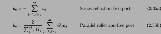
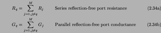
A useful simplification occurs when we can choose, for a particular port  (called a reflection-free port [57]) of an -port adaptor,
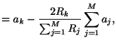
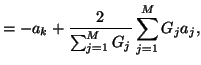
in which case the scattering equations (2.31) yield, for the output wave at port ,
Thus, at a reflection-free port , the output wave  is independent of the input wave
  ; such a port can be connected to any other without risk of a resulting delay-free loop. The same choices of port resistances (2.35) will also give a reflection-free port if power wave variables are employed.
Subsections
Next: Scattering Matrices for Adaptors
Up: Wave Digital Elements and
Previous: The Unit Element
Stefan Bilbao
2002-01-22