Next: Pseudopower and Pseudopassivity
Up: Wave Digital Elements and
Previous: The Bilinear Transform
Wave Variables
At this point, one may assume that we have finished; indeed, we can derive a discrete-time equivalent to any LTI  -port (graphically represented by a signal flow diagram involving shifts and arithmetic operations), and such elements can be connected using Kirchoff's Laws, which remain unchanged by the mapping (2.11). In particular, a network consisting of a collection of connected passive -ports will possess a discrete equivalent of the passivity property, which has been called pseudopassivity [42]. The problem, however, is that a simple application of the bilinear transform to a given -port usually leaves us with port variables which are not related to each other in a strictly causal way. For example, the difference equation (2.13) that results in the case of the inductor relates
  to
to  at every time step
  so that if we try to connect such a discrete-time one-port to another which has the same property (using Kirchoff's Laws, which are memoryless), we necessarily end up with non-realizable delay-free loops [46] in our resulting signal flow diagram. In other words, we will not be able to explicitly update all the port variables in our algorithm using only past values stored in the delay registers.
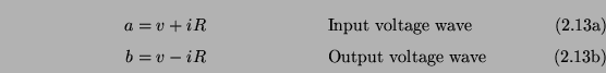
The problem of these delay-free loops was solved by Fettweis [41] with the introduction of wave variables, a concept with a long history borrowed from microwave electronics [11,12]. For a port with voltage  and current
  , voltage waves are defined by
 and
and  are referred to as wave variables, and in particular, is called an input wave and an output wave; the significance of these names will become clear in the examples of §2.3.4. This definition holds instantaneously, and will also be true for continuous and , though we will almost never have occasion to refer to analog wave variables in this thesis. The parameter
  is a free parameter known as the port resistance--its choice is governed by the character of the element itself. We also can define the port conductance
  by
by
 |
(2.15) |
at a port with port resistance  .
.
It is also possible to define power-normalized waves [46]
 and
and
 at any port with port resistance by
The two types of waves are simply related to each other by
 |
(2.17a) |
but power-normalized quantities have certain advantages in cases for which a port resistance is time-varying or signal dependent (indeed, in these cases, power-normalized waves must be employed if passivity in the digital simulation is to be maintained). In general, however, in view of (2.17), it should be assumed that we are using voltage waves unless otherwise indicated.
The steady state quantities  and
and  are defined in a manner identical to (2.14), where we replace and by
  and
and  .
.
Next: Pseudopower and Pseudopassivity
Up: Wave Digital Elements and
Previous: The Bilinear Transform
Stefan Bilbao
2002-01-22