The Bilinear Transform

Wave digital filters result from the mapping of a lumped analog electrical network (usually made up of the elements mentioned in the previous section connected using Kirchoff's Laws, and which is intended for use as a filter) into the discrete-time domain. In the linear time-invariant case, this translation is carried out using a particular type of spectral mapping between the analog frequency variable $s$ and a new discrete frequency variable $\psi$ which will be a rational function of $z^{-1} = e^{-sT}$ which is interpreted as a unit delay, of duration $T$; the mapping affects only reactive $N$-ports, i.e., those whose behavior is frequency-dependent, such as the inductor and capacitor. Memoryless elements, such as the transformer, gyrator and resistor (as well as the parallel or series connection, interpreted as an $N$-port) are frequency-independent, and will be unaffected by such a transformation.

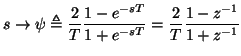
The frequency mapping proposed by Fettweis in [41] is a particular type of bilinear transform, given by

$$s\rightarrow \psi \triangleq \frac{2}{T}\frac{1-e^{-sT}}{1+e^{-sT}} = \frac{2}{T}\frac{1-z^{-1}}{1+z^{-1}}$$ (2.11)

We can then write

$${\rm Re}(\psi) = \frac{2}{T}\frac{1-e^{-2{\rm Re}(s)T}}{\vert 1+e^{-sT}\vert^{2}} = \frac{2}{T}\frac{1-\vert z\vert^{-2}}{\vert 1+z^{-1}\vert^{2}}$$

so clearly

$${\rm Re}(s)>0 \Longleftrightarrow {\rm Re}(\psi)> 0 \Longleftrightarrow \vert z\vert>1\notag$$

$${\rm Re}(s)<0 \Longleftrightarrow {\rm Re}(\psi)< 0 \Longleftrightarrow \vert z\vert<1$$

$${\rm Re}(s)=0 \Longleftrightarrow {\rm Re}(\psi)= 0 \Longleftrightarrow \vert z\vert=1\notag$$

Figure 2.6: Spectral mapping corresponding to the trapezoid rule.

This implies that stable, causal transfer functions in $s$ will be mapped to stable causal transfer functions in the discrete variable $z^{-1}$, and moreover that positive real functions will be mapped to functions which are positive real in the outer disk [162]. Such functions are often called pseudopassive [42], and have an energetic interpretation similar to that of their counterparts in the analog domain. (Indeed, Fettweis views pseudopassivity as simply passivity using a warped frequency variable $\psi$ [46].)

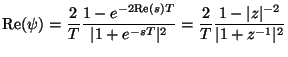In particular, for a harmonic state--that is, for real frequencies $\omega$ such that $s=j\omega$ and $z = e^{j\omega T}$, we have that

$$\omega\rightarrow \frac{2}{T}\tan\left(\frac{\omega T}{2}\right)$$ (2.12)

so that the entire analog frequency spectrum is mapped to the discrete frequency spectrum exactly once. In particular, we have that the analog DC frequency $s=0$ is mapped to discrete DC $z=1$, and that analog infinite frequency is mapped to the Nyquist frequency. It should be clear that there will be significant warping of the spectrum away from either extreme.

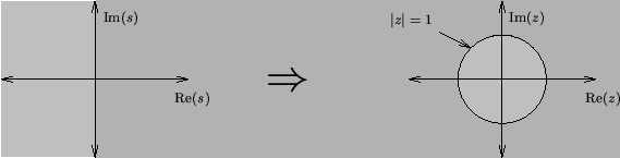
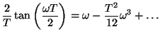
It is also worthwhile examining the mapping (2.11) on the unit circle in the low-frequency limit, in which case we can expand the right side of the mapping about $\omega = 0$, to get

$$\frac{2}{T}\tan\left(\frac{\omega T}{2}\right) = \omega - \frac{T^{2}}{12}\omega^{3}+\hdots$$

The mapping (2.12) can be rewritten as

$$\omega\rightarrow \omega + O(\omega^{3}T^{2})$$

The frequency mapping thus becomes more accurate near $\omega = 0$ in the limit as $T\rightarrow 0$. The order of this approximation (namely to $T^{2}$) will play an important role in numerical integration methods, because it defines the accuracy of a numerical scheme [65,131,176].

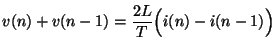
It is important to mention that the time-domain interpretation of the bilinear mapping (2.11) is called the trapezoid rule for numerical integration. That is, treating $z^{-1}$ as the unit delay, the right-hand side of (2.11) serves as an approximation to the derivative in a discrete-time setting. For example, in the case of the inductor, application of the mapping yields the following difference equation relating the voltage and current:

$$v(n) + v(n-1) = \frac{2L}{T}\Big(i(n)-i(n-1)\Big)$$ (2.13)

It should be understood here that $v(n)$ and $i(n)$ in (2.13) now represent discrete approximations to the voltage and current of (2.7) at time $t = nT$, for integer $n$. Generalizations of the WDF approach to cases in which the $N$-port of interest is time-varying or non-linear are based on this time-domain formulation, because in these cases, we no longer have a well-defined notion of frequency.

For the rest of this section, so as to avoid unnecessary extra notation, we will assume that we have discrete time voltages and currents. Thus $v$ and $i$ now refer to sequences $v(n)$ and $i(n)$, for $n$ integer, and the steady state quantities $\hat{v}$ and $\hat{i}$ are complex amplitudes of a sequence at the discrete frequency $z$.